AR(1) Processes - A First Course in Quantitative Economics with Python

32.1Overview¶

In this lecture we are going to study a very simple class of stochastic models called AR(1) processes.

These simple models are used again and again in economic research to represent the dynamics of series such as

labor income
dividends
productivity, etc.

We are going to study AR(1) processes partly because they are useful and partly because they help us understand important concepts.

Let’s start with some imports:

import numpy as np
import matplotlib.pyplot as plt
plt.rcParams["figure.figsize"] = (11, 5)  #set default figure size

32.2The AR(1) model¶

The AR(1) model (autoregressive model of order 1) takes the form

X_{t+1} = a X_t + b + c W_{t+1}

(1)

where $a, b, c$ are scalar-valued parameters

(Equation (1) is sometimes called a stochastic difference equation.)

The specification (1) generates a time series $\{ X_t\}$ as soon as we specify an initial condition $X_0$ .

To make things even simpler, we will assume that

the process $\{ W_t \}$ is IID and standard normal,
the initial condition $X_0$ is drawn from the normal distribution $N(\mu_0, v_0)$ and
the initial condition $X_0$ is independent of $\{ W_t \}$ .

32.2.1Moving average representation¶

Iterating backwards from time $t$ , we obtain

X_t = a X_{t-1} + b + c W_t = a^2 X_{t-2} + a b + a c W_{t-1} + b + c W_t = a^3 X_{t-3} + a^2 b + a^2 c W_{t-2} + b + c W_t = \cdots

(2)

If we work all the way back to time zero, we get

X_t = a^t X_0 + b \sum_{j=0}^{t-1} a^j + c \sum_{j=0}^{t-1} a^j W_{t-j}

(3)

Equation (3) shows that $X_t$ is a well defined random variable, the value of which depends on

the parameters,
the initial condition $X_0$ and
the shocks $W_1, \ldots W_t$ from time $t=1$ to the present.

Throughout, the symbol $\psi_t$ will be used to refer to the density of this random variable $X_t$ .

32.2.2Distribution dynamics¶

One of the nice things about this model is that it’s so easy to trace out the sequence of distributions $\{ \psi_t \}$ corresponding to the time series $\{ X_t\}$ .

To see this, we first note that $X_t$ is normally distributed for each $t$ .

This is immediate from (3), since linear combinations of independent normal random variables are normal.

Given that $X_t$ is normally distributed, we will know the full distribution $\psi_t$ if we can pin down its first two moments.

Let $\mu_t$ and $v_t$ denote the mean and variance of $X_t$ respectively.

We can pin down these values from (3) or we can use the following recursive expressions:

\mu_{t+1} = a \mu_t + b \quad \text{and} \quad v_{t+1} = a^2 v_t + c^2

(4)

These expressions are obtained from (1) by taking, respectively, the expectation and variance of both sides of the equality.

In calculating the second expression, we are using the fact that $X_t$ and $W_{t+1}$ are independent.

(This follows from our assumptions and (3).)

Given the dynamics in (3) and initial conditions $\mu_0, v_0$ , we obtain $\mu_t, v_t$ and hence

\psi_t = N(\mu_t, v_t)

(5)

The following code uses these facts to track the sequence of marginal distributions $\{ \psi_t \}$ .

The parameters are

a, b, c = 0.9, 0.1, 0.5

mu, v = -3.0, 0.6  # initial conditions mu_0, v_0

Here’s the sequence of distributions:

from scipy.stats import norm

sim_length = 10
grid = np.linspace(-5, 7, 120)

fig, ax = plt.subplots()

for t in range(sim_length):
    mu = a * mu + b
    v = a**2 * v + c**2
    ax.plot(grid, norm.pdf(grid, loc=mu, scale=np.sqrt(v)),
            label=fr"$\psi_{t}$",
            alpha=0.7)

ax.legend(bbox_to_anchor=[1.05,1],loc=2,borderaxespad=1)

plt.show()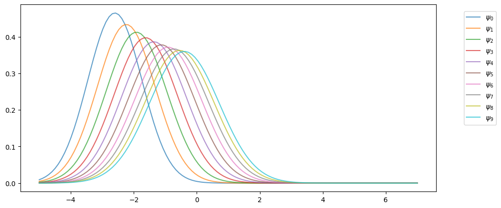

32.3Stationarity and asymptotic stability¶

When we use models to study the real world, it is generally preferable that our models have clear, sharp predictions.

For dynamic problems, sharp predictions are related to stability.

For example, if a dynamic model predicts that inflation always converges to some kind of steady state, then the model gives a sharp prediction.

(The prediction might be wrong, but even this is helpful, because we can judge the quality of the model.)

Notice that, in the figure above, the sequence $\{ \psi_t \}$ seems to be converging to a limiting distribution, suggesting some kind of stability.

This is even clearer if we project forward further into the future:

def plot_density_seq(ax, mu_0=-3.0, v_0=0.6, sim_length=40):
    mu, v = mu_0, v_0
    for t in range(sim_length):
        mu = a * mu + b
        v = a**2 * v + c**2
        ax.plot(grid,
                norm.pdf(grid, loc=mu, scale=np.sqrt(v)),
                alpha=0.5)

fig, ax = plt.subplots()
plot_density_seq(ax)
plt.show()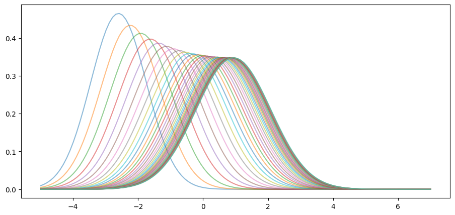

Moreover, the limit does not depend on the initial condition.

For example, this alternative density sequence also converges to the same limit.

fig, ax = plt.subplots()
plot_density_seq(ax, mu_0=4.0)
plt.show()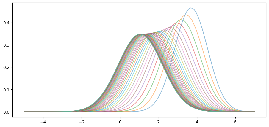

In fact it’s easy to show that such convergence will occur, regardless of the initial condition, whenever $|a| < 1$ .

To see this, we just have to look at the dynamics of the first two moments, as given in (4).

When $|a| < 1$ , these sequences converge to the respective limits

\mu^* := \frac{b}{1-a} \quad \text{and} \quad v^* = \frac{c^2}{1 - a^2}

(6)

(See our lecture on one dimensional dynamics for background on deterministic convergence.)

Hence

\psi_t \to \psi^* = N(\mu^*, v^*) \quad \text{as } t \to \infty

(7)

We can confirm this is valid for the sequence above using the following code.

fig, ax = plt.subplots()
plot_density_seq(ax, mu_0=4.0)

mu_star = b / (1 - a)
std_star = np.sqrt(c**2 / (1 - a**2))  # square root of v_star
psi_star = norm.pdf(grid, loc=mu_star, scale=std_star)
ax.plot(grid, psi_star, 'k-', lw=2, label=r"$\psi^*$")
ax.legend()

plt.show()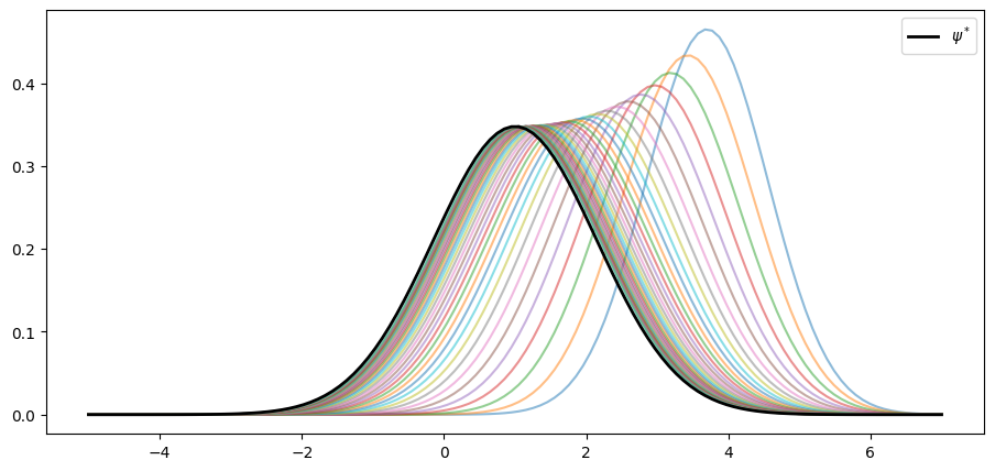

As claimed, the sequence $\{ \psi_t \}$ converges to $\psi^*$ .

We see that, at least for these parameters, the AR(1) model has strong stability properties.

32.3.1Stationary distributions¶

Let’s try to better understand the limiting distribution $\psi^*$ .

A stationary distribution is a distribution that is a “fixed point” of the update rule for the AR(1) process.

In other words, if $\psi_t$ is stationary, then $\psi_{t+j} = \psi_t$ for all $j$ in $\mathbb N$ .

A different way to put this, specialized to the current setting, is as follows: a density ψ on $\mathbb R$ is stationary for the AR(1) process if

X_t \sim \psi \quad \implies \quad a X_t + b + c W_{t+1} \sim \psi

(8)

The distribution $\psi^*$ in (7) has this property --- checking this is an exercise.

(Of course, we are assuming that $|a| < 1$ so that $\psi^*$ is well defined.)

In fact, it can be shown that no other distribution on $\mathbb R$ has this property.

Thus, when $|a| < 1$ , the AR(1) model has exactly one stationary density and that density is given by $\psi^*$ .

32.4Ergodicity¶

The concept of ergodicity is used in different ways by different authors.

One way to understand it in the present setting is that a version of the law of large numbers is valid for $\{X_t\}$ , even though it is not IID.

In particular, averages over time series converge to expectations under the stationary distribution.

Indeed, it can be proved that, whenever $|a| < 1$ , we have

\frac{1}{m} \sum_{t = 1}^m h(X_t) \to \int h(x) \psi^*(x) dx \quad \text{as } m \to \infty

(9)

whenever the integral on the right hand side is finite and well defined.

Notes:

In (9), convergence holds with probability one.
The textbook by Meyn & Tweedie (2009) is a classic reference on ergodicity.

Ergodicity is important for a range of reasons.

For example, (9) can be used to test theory.

In this equation, we can use observed data to evaluate the left hand side of (9).

And we can use a theoretical AR(1) model to calculate the right hand side.

If $\frac{1}{m} \sum_{t = 1}^m X_t$ is not close to $\psi^(x)$ , even for many observations, then our theory seems to be incorrect and we will need to revise it.

32.5Exercises¶

Exercise 1

Let $k$ be a natural number.

The $k$ -th central moment of a random variable is defined as

M_k := \mathbb E [ (X - \mathbb E X )^k ]

(11)

When that random variable is $N(\mu, \sigma^2)$ , it is known that

M_k = \begin{cases} 0 & \text{ if } k \text{ is odd} \\ \sigma^k (k-1)!! & \text{ if } k \text{ is even} \end{cases}

(12)

Here $n!!$ is the double factorial.

According to (9), we should have, for any $k \in \mathbb N$ ,

\frac{1}{m} \sum_{t = 1}^m (X_t - \mu^* )^k \approx M_k

(13)

when $m$ is large.

Confirm this by simulation at a range of $k$ using the default parameters from the lecture.

Solution to Exercise 1

Here is one solution:

from numba import njit
from scipy.special import factorial2

@njit
def sample_moments_ar1(k, m=100_000, mu_0=0.0, sigma_0=1.0, seed=1234):
    np.random.seed(seed)
    sample_sum = 0.0
    x = mu_0 + sigma_0 * np.random.randn()
    for t in range(m):
        sample_sum += (x - mu_star)**k
        x = a * x + b + c * np.random.randn()
    return sample_sum / m

def true_moments_ar1(k):
    if k % 2 == 0:
        return std_star**k * factorial2(k - 1)
    else:
        return 0

k_vals = np.arange(6) + 1
sample_moments = np.empty_like(k_vals)
true_moments = np.empty_like(k_vals)

for k_idx, k in enumerate(k_vals):
    sample_moments[k_idx] = sample_moments_ar1(k)
    true_moments[k_idx] = true_moments_ar1(k)

fig, ax = plt.subplots()
ax.plot(k_vals, true_moments, label="true moments")
ax.plot(k_vals, sample_moments, label="sample moments")
ax.legend()

plt.show()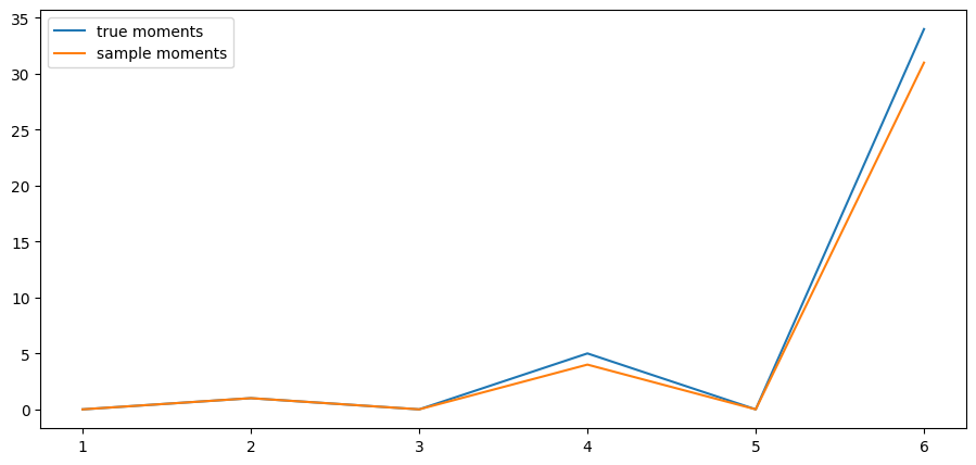

Exercise 2

Write your own version of a one dimensional kernel density estimator, which estimates a density from a sample.

Write it as a class that takes the data $X$ and bandwidth $h$ when initialized and provides a method $f$ such that

f(x) = \frac{1}{hn} \sum_{i=1}^n K \left( \frac{x-X_i}{h} \right)

(14)

For $K$ use the Gaussian kernel ( $K$ is the standard normal density).

Write the class so that the bandwidth defaults to Silverman’s rule (see the “rule of thumb” discussion on this page). Test the class you have written by going through the steps

simulate data $X_1, \ldots, X_n$ from distribution ϕ
plot the kernel density estimate over a suitable range
plot the density of ϕ on the same figure

for distributions ϕ of the following types

beta distribution with $\alpha = \beta = 2$
beta distribution with $\alpha = 2$ and $\beta = 5$
beta distribution with $\alpha = \beta = 0.5$

Use $n=500$ .

Make a comment on your results. (Do you think this is a good estimator of these distributions?)

Solution to Exercise 2

Here is one solution:

K = norm.pdf

class KDE:

    def __init__(self, x_data, h=None):

        if h is None:
            c = x_data.std()
            n = len(x_data)
            h = 1.06 * c * n**(-1/5)
        self.h = h
        self.x_data = x_data

    def f(self, x):
        if np.isscalar(x):
            return K((x - self.x_data) / self.h).mean() * (1/self.h)
        else:
            y = np.empty_like(x)
            for i, x_val in enumerate(x):
                y[i] = K((x_val - self.x_data) / self.h).mean() * (1/self.h)
            return y

def plot_kde(ϕ, x_min=-0.2, x_max=1.2):
    x_data = ϕ.rvs(n)
    kde = KDE(x_data)

    x_grid = np.linspace(-0.2, 1.2, 100)
    fig, ax = plt.subplots()
    ax.plot(x_grid, kde.f(x_grid), label="estimate")
    ax.plot(x_grid, ϕ.pdf(x_grid), label="true density")
    ax.legend()
    plt.show()

from scipy.stats import beta

n = 500
parameter_pairs= (2, 2), (2, 5), (0.5, 0.5)
for α, β in parameter_pairs:
    plot_kde(beta(α, β))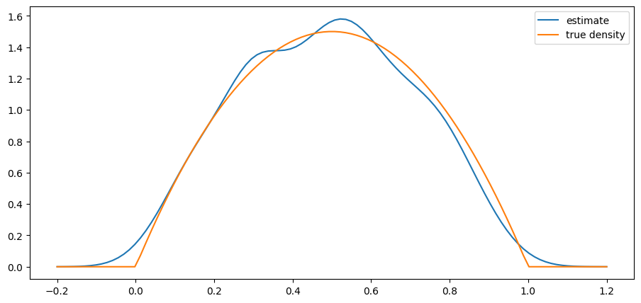

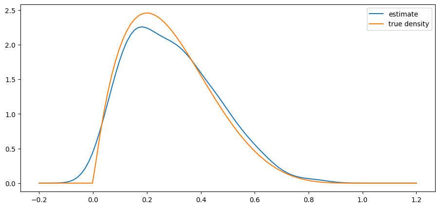
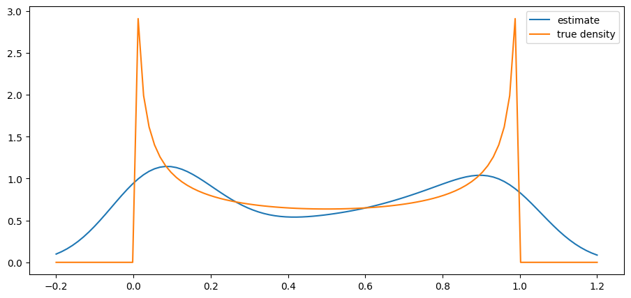
We see that the kernel density estimator is effective when the underlying distribution is smooth but less so otherwise.

Exercise 3

In the lecture we discussed the following fact: for the $AR(1)$ process

X_{t+1} = a X_t + b + c W_{t+1}

(15)

with $\{ W_t \}$ iid and standard normal,

\psi_t = N(\mu, s^2) \implies \psi_{t+1} = N(a \mu + b, a^2 s^2 + c^2)

(16)

Confirm this, at least approximately, by simulation. Let

$a = 0.9$
$b = 0.0$
$c = 0.1$
$\mu = -3$
$s = 0.2$

First, plot $\psi_t$ and $\psi_{t+1}$ using the true distributions described above.

Second, plot $\psi_{t+1}$ on the same figure (in a different color) as follows:

Generate $n$ draws of $X_t$ from the $N(\mu, s^2)$ distribution
Update them all using the rule $X_{t+1} = a X_t + b + c W_{t+1}$
Use the resulting sample of $X_{t+1}$ values to produce a density estimate via kernel density estimation.

Try this for $n=2000$ and confirm that the simulation based estimate of $\psi_{t+1}$ does converge to the theoretical distribution.

Solution to Exercise 3

Here is our solution

a = 0.9
b = 0.0
c = 0.1
μ = -3
s = 0.2

μ_next = a * μ + b
s_next = np.sqrt(a**2 * s**2 + c**2)

ψ = lambda x: K((x - μ) / s)
ψ_next = lambda x: K((x - μ_next) / s_next)

ψ = norm(μ, s)
ψ_next = norm(μ_next, s_next)

n = 2000
x_draws = ψ.rvs(n)
x_draws_next = a * x_draws + b + c * np.random.randn(n)
kde = KDE(x_draws_next)

x_grid = np.linspace(μ - 1, μ + 1, 100)
fig, ax = plt.subplots()

ax.plot(x_grid, ψ.pdf(x_grid), label="$\psi_t$")
ax.plot(x_grid, ψ_next.pdf(x_grid), label="$\psi_{t+1}$")
ax.plot(x_grid, kde.f(x_grid), label="estimate of $\psi_{t+1}$")

ax.legend()
plt.show()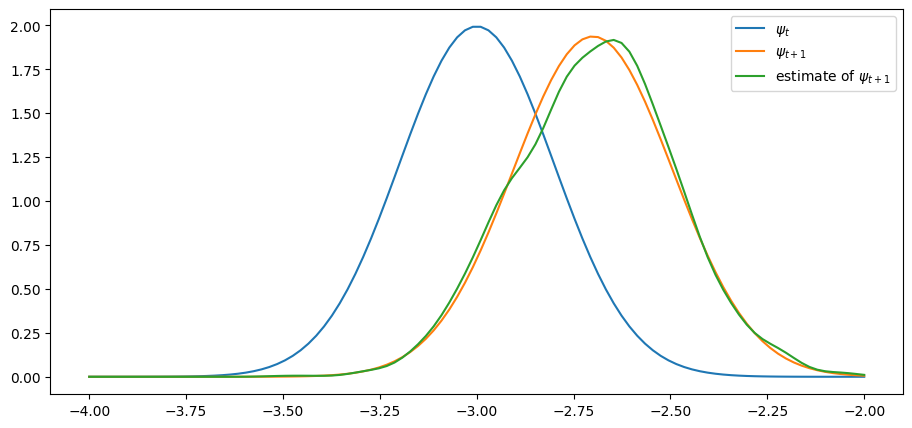

The simulated distribution approximately coincides with the theoretical distribution, as predicted.