Maximum Likelihood Estimation - A First Course in Quantitative Economics with Python

from scipy.stats import lognorm, pareto, expon
import numpy as np
from scipy.integrate import quad
import matplotlib.pyplot as plt
import pandas as pd
from math import exp

45.1Introduction¶

Consider a situation where a policymaker is trying to estimate how much revenue a proposed wealth tax will raise.

The proposed tax is

h(w) = \begin{cases} a w & \text{if } w \leq \bar w \\ a \bar{w} + b (w-\bar{w}) & \text{if } w > \bar w \end{cases}

(1)

where $w$ is wealth.

Let’s go ahead and define $h$ :

def h(w, a=0.05, b=0.1, w_bar=2.5):
    if w <= w_bar:
        return a * w
    else:
        return a * w_bar + b * (w - w_bar)

For a population of size $N$ , where individual $i$ has wealth $w_i$ , total revenue raised by the tax will be

T = \sum_{i=1}^{N} h(w_i)

(2)

We wish to calculate this quantity.

The problem we face is that, in most countries, wealth is not observed for all individuals.

Collecting and maintaining accurate wealth data for all individuals or households in a country is just too hard.

So let’s suppose instead that we obtain a sample $w_1, w_2, \cdots, w_n$ telling us the wealth of $n$ randomly selected individuals.

For our exercise we are going to use a sample of $n = 10,000$ observations from wealth data in the US in 2016.

n = 10_000

The data is derived from the Survey of Consumer Finances (SCF).

The following code imports this data and reads it into an array called sample.

Source

url = 'https://media.githubusercontent.com/media/QuantEcon/high_dim_data/update_scf_noweights/SCF_plus/SCF_plus_mini_no_weights.csv'
df = pd.read_csv(url)
df = df.dropna()
df = df[df['year'] == 2016]
df = df.loc[df['n_wealth'] > 1 ]   #restrcting data to net worth > 1
rv = df['n_wealth'].sample(n=n, random_state=1234)
rv = rv.to_numpy() / 100_000
sample = rv

Let’s histogram this sample.

fig, ax = plt.subplots()
ax.set_xlim(-1, 20)
density, edges = np.histogram(sample, bins=5000, density=True)
prob = density * np.diff(edges)
plt.stairs(prob, edges, fill=True, alpha=0.8, label=r"unit: $\$100,000$")
plt.ylabel("prob")
plt.xlabel("net wealth")
plt.legend()
plt.show()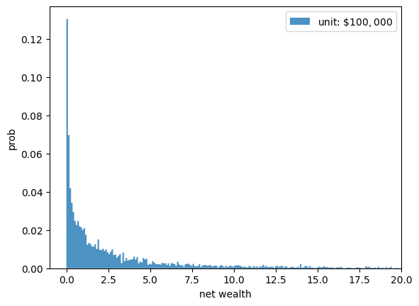

The histogram shows that many people have very low wealth and a few people have very high wealth.

We will take the full population size to be

N = 100_000_000

How can we estimate total revenue from the full population using only the sample data?

Our plan is to assume that wealth of each individual is a draw from a distribution with density $f$ .

If we obtain an estimate of $f$ we can then approximate $T$ as follows:

T = \sum_{i=1}^{N} h(w_i) = N \frac{1}{N} \sum_{i=1}^{N} h(w_i) \approx N \int_{0}^{\infty} h(w)f(w) dw

(3)

(The sample mean should be close to the mean by the law of large numbers.)

The problem now is: how do we estimate $f$ ?

45.2Maximum likelihood estimation¶

Maximum likelihood estimation is a method of estimating an unknown distribution.

Maximum likelihood estimation has two steps:

Guess what the underlying distribution is (e.g., normal with mean μ and standard deviation σ).
Estimate the parameter values (e.g., estimate μ and σ for the normal distribution)

One possible assumption for the wealth is that each $w_i$ is log-normally distributed, with parameters $\mu \in (-\infty,\infty)$ and $\sigma \in (0,\infty)$ .

(This means that $\ln w_i$ is normally distributed with mean μ and standard deviation σ.)

You can see that this assumption is not completely unreasonable because, if we histogram log wealth instead of wealth, the picture starts to look something like a bell-shaped curve.

ln_sample = np.log(sample)
fig, ax = plt.subplots()
ax.hist(ln_sample, density=True, bins=200, histtype='stepfilled', alpha=0.8)
plt.show()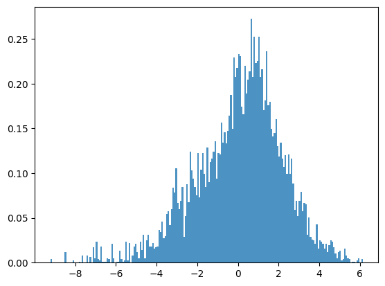

Now our job is to obtain the maximum likelihood estimates of μ and σ, which we denote by $\hat{\mu}$ and $\hat{\sigma}$ .

These estimates can be found by maximizing the likelihood function given the data.

The pdf of a lognormally distributed random variable $X$ is given by:

f(x, \mu, \sigma) = \frac{1}{x}\frac{1}{\sigma \sqrt{2\pi}} \exp\left(\frac{-1}{2}\left(\frac{\ln x-\mu}{\sigma}\right)\right)^2

(4)

For our sample $w_1, w_2, \cdots, w_n$ , the likelihood function is given by

L(\mu, \sigma | w_i) = \prod_{i=1}^{n} f(w_i, \mu, \sigma)

(5)

The likelihood function can be viewed as both

the joint distribution of the sample (which is assumed to be IID) and
the “likelihood” of parameters $(\mu, \sigma)$ given the data.

Taking logs on both sides gives us the log likelihood function, which is

\begin{aligned} \ell(\mu, \sigma | w_i) & = \ln \left[ \prod_{i=1}^{n} f(w_i, \mu, \sigma) \right] \\ & = -\sum_{i=1}^{n} \ln w_i - \frac{n}{2} \ln(2\pi) - \frac{n}{2} \ln \sigma^2 - \frac{1}{2\sigma^2} \sum_{i=1}^n (\ln w_i - \mu)^2 \end{aligned}

(6)

To find where this function is maximised we find its partial derivatives wrt μ and $\sigma ^2$ and equate them to 0.

Let’s first find the maximum likelihood estimate (MLE) of μ

\frac{\delta \ell}{\delta \mu} = - \frac{1}{2\sigma^2} \times 2 \sum_{i=1}^n (\ln w_i - \mu) = 0 \\ \implies \sum_{i=1}^n \ln w_i - n \mu = 0 \\ \implies \hat{\mu} = \frac{\sum_{i=1}^n \ln w_i}{n}

(7)

Now let’s find the MLE of σ

\frac{\delta \ell}{\delta \sigma^2} = - \frac{n}{2\sigma^2} + \frac{1}{2\sigma^4} \sum_{i=1}^n (\ln w_i - \mu)^2 = 0 \\ \implies \frac{n}{2\sigma^2} = \frac{1}{2\sigma^4} \sum_{i=1}^n (\ln w_i - \mu)^2 \\ \implies \hat{\sigma} = \left( \frac{\sum_{i=1}^{n}(\ln w_i - \hat{\mu})^2}{n} \right)^{1/2}

(8)

Now that we have derived the expressions for $\hat{\mu}$ and $\hat{\sigma}$ , let’s compute them for our wealth sample.

μ_hat = np.mean(ln_sample)
μ_hat

np.float64(0.0634375526654064)

num = (ln_sample - μ_hat)**2
σ_hat = (np.mean(num))**(1/2)
σ_hat

np.float64(2.1507346258433424)

Let’s plot the lognormal pdf using the estimated parameters against our sample data.

dist_lognorm = lognorm(σ_hat, scale = exp(μ_hat))
x = np.linspace(0,50,10000)

fig, ax = plt.subplots()
ax.set_xlim(-1,20)

ax.hist(sample, density=True, bins=5_000, histtype='stepfilled', alpha=0.5)
ax.plot(x, dist_lognorm.pdf(x), 'k-', lw=0.5, label='lognormal pdf')
ax.legend()
plt.show()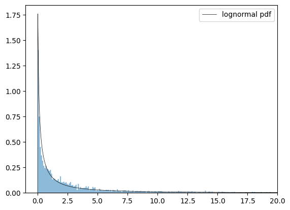

Our estimated lognormal distribution appears to be a reasonable fit for the overall data.

We now use (3) to calculate total revenue.

We will compute the integral using numerical integration via SciPy’s quad function

def total_revenue(dist):
    integral, _ = quad(lambda x: h(x) * dist.pdf(x), 0, 100_000)
    T = N * integral
    return T

tr_lognorm = total_revenue(dist_lognorm)
tr_lognorm

101105326.82814859

(Our unit was 100,000 dollars, so this means that actual revenue is 100,000 times as large.)

45.3Pareto distribution¶

We mentioned above that using maximum likelihood estimation requires us to make a prior assumption of the underlying distribution.

Previously we assumed that the distribution is lognormal.

Suppose instead we assume that $w_i$ are drawn from the Pareto Distribution with parameters $b$ and $x_m$ .

In this case, the maximum likelihood estimates are known to be

\hat{b} = \frac{n}{\sum_{i=1}^{n} \ln (w_i/\hat{x_m})} \quad \text{and} \quad \hat{x}_m = \min_{i} w_i

(9)

Let’s calculate them.

xm_hat = min(sample)
xm_hat

np.float64(0.0001)

den = np.log(sample/xm_hat)
b_hat = 1/np.mean(den)
b_hat

np.float64(0.10783091940803055)

Now let’s recompute total revenue.

dist_pareto = pareto(b = b_hat, scale = xm_hat)
tr_pareto = total_revenue(dist_pareto) 
tr_pareto

12933168365.762571

The number is very different!

tr_pareto / tr_lognorm

127.91777418162567

We see that choosing the right distribution is extremely important.

Let’s compare the fitted Pareto distribution to the histogram:

fig, ax = plt.subplots()
ax.set_xlim(-1, 20)
ax.set_ylim(0,1.75)

ax.hist(sample, density=True, bins=5_000, histtype='stepfilled', alpha=0.5)
ax.plot(x, dist_pareto.pdf(x), 'k-', lw=0.5, label='Pareto pdf')
ax.legend()

plt.show()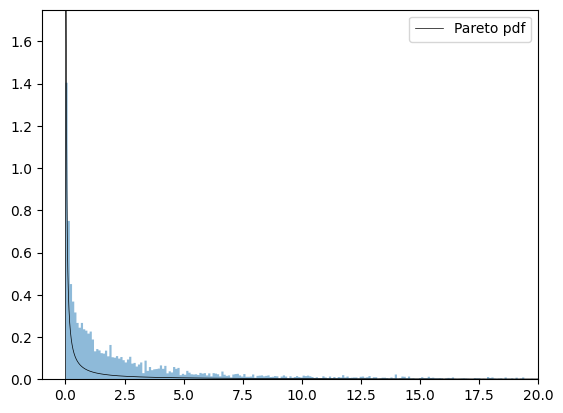

We observe that in this case the fit for the Pareto distribution is not very good, so we can probably reject it.

45.4What is the best distribution?¶

There is no “best” distribution --- every choice we make is an assumption.

All we can do is try to pick a distribution that fits the data well.

The plots above suggested that the lognormal distribution is optimal.

However when we inspect the upper tail (the richest people), the Pareto distribution may be a better fit.

To see this, let’s now set a minimum threshold of net worth in our dataset.

We set an arbitrary threshold of $500,000 and read the data into sample_tail.

Source

df_tail = df.loc[df['n_wealth'] > 500_000 ]
df_tail.head()
rv_tail = df_tail['n_wealth'].sample(n=10_000, random_state=4321)
rv_tail = rv_tail.to_numpy()
sample_tail = rv_tail/500_000

Let’s plot this data.

fig, ax = plt.subplots()
ax.set_xlim(0,50)
ax.hist(sample_tail, density=True, bins=500, histtype='stepfilled', alpha=0.8)
plt.show()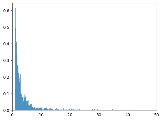

Now let’s try fitting some distributions to this data.

45.4.1Lognormal distribution for the right hand tail¶

Let’s start with the lognormal distribution

We estimate the parameters again and plot the density against our data.

ln_sample_tail = np.log(sample_tail)
μ_hat_tail = np.mean(ln_sample_tail)
num_tail = (ln_sample_tail - μ_hat_tail)**2
σ_hat_tail = (np.mean(num_tail))**(1/2)
dist_lognorm_tail = lognorm(σ_hat_tail, scale = exp(μ_hat_tail))

fig, ax = plt.subplots()
ax.set_xlim(0,50)
ax.hist(sample_tail, density=True, bins=500, histtype='stepfilled', alpha=0.5)
ax.plot(x, dist_lognorm_tail.pdf(x), 'k-', lw=0.5, label='lognormal pdf')
ax.legend()
plt.show()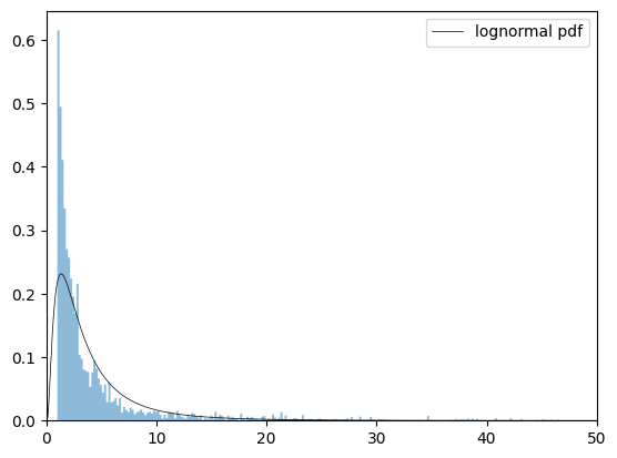

While the lognormal distribution was a good fit for the entire dataset, it is not a good fit for the right hand tail.

45.4.2Pareto distribution for the right hand tail¶

Let’s now assume the truncated dataset has a Pareto distribution.

We estimate the parameters again and plot the density against our data.

xm_hat_tail = min(sample_tail)
den_tail = np.log(sample_tail/xm_hat_tail)
b_hat_tail = 1/np.mean(den_tail)
dist_pareto_tail = pareto(b = b_hat_tail, scale = xm_hat_tail)

fig, ax = plt.subplots()
ax.set_xlim(0, 50)
ax.set_ylim(0,0.65)
ax.hist(sample_tail, density=True, bins= 500, histtype='stepfilled', alpha=0.5)
ax.plot(x, dist_pareto_tail.pdf(x), 'k-', lw=0.5, label='pareto pdf')
plt.show()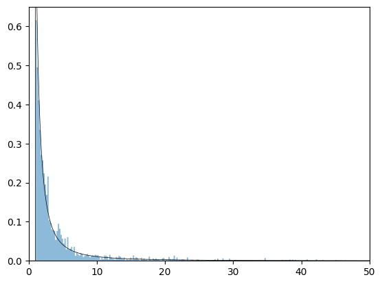

The Pareto distribution is a better fit for the right hand tail of our dataset.

45.4.3So what is the best distribution?¶

As we said above, there is no “best” distribution --- each choice is an assumption.

We just have to test what we think are reasonable distributions.

One test is to plot the data against the fitted distribution, as we did.

There are other more rigorous tests, such as the Kolmogorov-Smirnov test.

We omit such advanced topics (but encourage readers to study them once they have completed these lectures).

45.5Exercises¶

Solution to Exercise 1

λ_hat = 1/np.mean(sample)
λ_hat

np.float64(0.15234120963403971)

dist_exp = expon(scale = 1/λ_hat)
tr_expo = total_revenue(dist_exp) 
tr_expo

55246978.53427645

Solution to Exercise 2

fig, ax = plt.subplots()
ax.set_xlim(-1, 20)

ax.hist(sample, density=True, bins=5000, histtype='stepfilled', alpha=0.5)
ax.plot(x, dist_exp.pdf(x), 'k-', lw=0.5, label='exponential pdf')
ax.legend()

plt.show()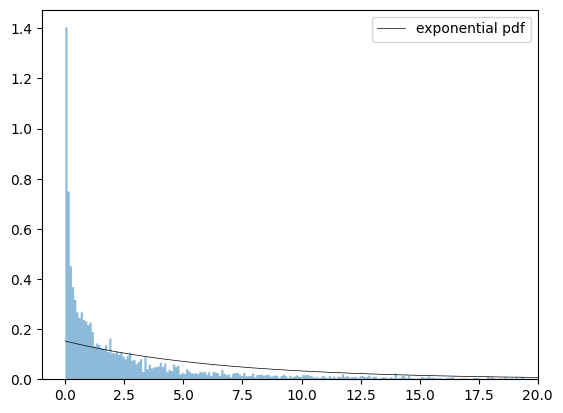

Clearly, this distribution is not a good fit for our data.