Laffer Curves with Adaptive Expectations - A First Course in Quantitative Economics with Python

A First Course in Quantitative Economics with Python

Laffer Curves with Adaptive Expectations

and

31.1Overview¶

This lecture studies stationary and dynamic Laffer curves in the inflation tax rate in a non-linear version of the model studied in this lecture Money Financed Government Deficits and Price Levels.

As in the lecture Money Financed Government Deficits and Price Levels, this lecture uses the log-linear version of the demand function for money that Cagan (1956) used in his classic paper in place of the linear demand function used in this lecture Money Financed Government Deficits and Price Levels.

But now, instead of assuming ‘‘rational expectations’’ in the form of ‘‘perfect foresight’’, we’ll adopt the ‘‘adaptive expectations’’ assumption used by Cagan (1956) and Friedman (1956).

This means that instead of assuming that expected inflation $\pi_t^*$ is described by the “perfect foresight” or “rational expectations” hypothesis

\pi_t^* = p_{t+1} - p_t

(1)

that we adopted in lectures Money Financed Government Deficits and Price Levels and lectures Inflation Rate Laffer Curves, we’ll now assume that $\pi_t^*$ is determined by the adaptive expectations hypothesis described in equation (5) reported below.

We shall discover that changing our hypothesis about expectations formation in this way will change some our findings and leave others intact. In particular, we shall discover that

replacing rational expectations with adaptive expectations leaves the two stationary inflation rates unchanged, but that $\ldots$
it reverses the perverse dynamics by making the lower stationary inflation rate the one to which the system typically converges
a more plausible comparative dynamic outcome emerges in which now inflation can be reduced by running lower government deficits

These more plausible comparative dynamics underlie the “old time religion” that states that “inflation is always and everywhere caused by government deficits”.

These issues were studied by Bruno & Fischer (1990).

Their purpose was to reverse what they thought were counter intuitive predictions of their model under rational expectations (i.e., perfect foresight in this context) by dropping rational expectations and instead assuming that people form expectations about future inflation rates according to the “adaptive expectations” scheme (5) described below.

31.2The model¶

Let

$m_t$ be the log of the money supply at the beginning of time $t$
$p_t$ be the log of the price level at time $t$
$\pi_t^*$ be the public’s expectation of the rate of inflation between $t$ and $t+1$

The law of motion of the money supply is

\exp(m_{t+1}) - \exp(m_t) = g \exp(p_t)

(2)

where $g$ is the part of government expenditures financed by printing money.

Notice that equation (2) implies that

m_{t+1} = \log[ \exp(m_t) + g \exp(p_t)]

(3)

The demand function for money is

m_{t+1} - p_t = -\alpha \pi_t^*

(4)

where $\alpha \geq 0$ .

Expectations of inflation are governed by

\pi_{t}^* = (1-\delta) (p_t - p_{t-1}) + \delta \pi_{t-1}^*

(5)

where $\delta \in (0,1)$

31.3Computing an equilibrium sequence¶

Equation the expressions for $m_{t+1}$ provided by (4) and (3) and use equation (5) to eliminate $\pi_t^*$ to obtain the following equation for $p_t$ :

\log[ \exp(m_t) + g \exp(p_t)] - p_t = -\alpha [(1-\delta) (p_t - p_{t-1}) + \delta \pi_{t-1}^*]

(6)

Pseudo-code

Here is the pseudo-code for our algorithm.

Starting at time 0 with initial conditions $(m_0, \pi_{-1}^*, p_{-1})$ , for each $t \geq 0$ deploy the following steps in order:

solve (6) for $p_t$
solve equation (5) for $\pi_t^*$
solve equation (3) for $m_{t+1}$

This completes the algorithm.

31.4Claims or conjectures¶

It will turn out that

if they exist, limiting values $\overline \pi$ and $\overline \mu$ will be equal
if limiting values exist, there are two possible limiting values, one high, one low
unlike the outcome in lecture Inflation Rate Laffer Curves, for almost all initial log price levels and expected inflation rates $p_0, \pi_{t}^*$ , the limiting $\overline \pi = \overline \mu$ is the lower steady state value
for each of the two possible limiting values $\bar \pi$ ,there is a unique initial log price level $p_0$ that implies that $\pi_t = \mu_t = \bar \mu$ for all $t \geq 0$
- this unique initial log price level solves $\log(\exp(m_0) + g \exp(p_0)) - p_0 = - \alpha \bar \pi$
- the preceding equation for $p_0$ comes from $m_1 - p_0 = - \alpha \bar \pi$

31.5Limiting values of inflation rate¶

As in our earlier lecture Inflation Rate Laffer Curves, we can compute the two prospective limiting values for $\bar \pi$ by studying the steady-state Laffer curve.

Thus, in a steady state

m_{t+1} - m_t = p_{t+1} - p_t = x \quad \forall t ,

(7)

where $x > 0$ is a common rate of growth of logarithms of the money supply and price level.

A few lines of algebra yields the following equation that $x$ satisfies

\exp(-\alpha x) - \exp(-(1 + \alpha) x) = g

(8)

where we require that

g \leq \max_{x: x \geq 0} \exp(-\alpha x) - \exp(-(1 + \alpha) x) ,

(9)

so that it is feasible to finance $g$ by printing money.

The left side of (8) is steady state revenue raised by printing money.

The right side of (8) is the quantity of time $t$ goods that the government raises by printing money.

Soon we’ll plot the left and right sides of equation (8).

But first we’ll write code that computes a steady-state $\bar \pi$ .

Let’s start by importing some libraries

from collections import namedtuple
import numpy as np
import matplotlib.pyplot as plt
from matplotlib.ticker import MaxNLocator
from matplotlib.cm import get_cmap
from matplotlib.colors import to_rgba
import matplotlib
from scipy.optimize import root, fsolve

Let’s create a namedtuple to store the parameters of the model

LafferAdaptive = namedtuple('LafferAdaptive', 
                        ["m0",  # log of the money supply at t=0
                         "α",   # sensitivity of money demand
                         "g",   # government expenditure
                         "δ"])

# Create a Cagan Laffer model
def create_model(α=0.5, m0=np.log(100), g=0.35, δ=0.9):
    return LafferAdaptive(α=α, m0=m0, g=g, δ=δ)

model = create_model()

Now we write code that computes steady-state $\bar \pi$ s.

# Define formula for π_bar
def solve_π(x, α, g):
    return np.exp(-α * x) - np.exp(-(1 + α) * x) - g

def solve_π_bar(model, x0):
    π_bar = fsolve(solve_π, x0=x0, xtol=1e-10, args=(model.α, model.g))[0]
    return π_bar

# Solve for the two steady state of π
π_l = solve_π_bar(model, x0=0.6)
π_u = solve_π_bar(model, x0=3.0)
print(f'The two steady state of π are: {π_l, π_u}')

The two steady state of π are: (np.float64(0.6737147075333034), np.float64(1.6930797322614815))

We find two steady state $\bar \pi$ values

31.6Steady-state Laffer curve¶

The following figure plots the steady-state Laffer curve together with the two stationary inflation rates.

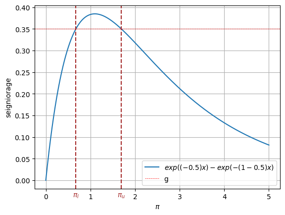
<Figure size 640x480 with 1 Axes> — Figure 1:Seigniorage as function of steady-state inflation. The dashed brown lines indicate $\pi_l$ and $\pi_u$ .

31.7Associated initial price levels¶

Now that we have our hands on the two possible steady states, we can compute two initial log price levels $p_{-1}$ , which as initial conditions, imply that $\pi_t = \bar \pi$ for all $t \geq 0$ .

In particular, to initiate a fixed point of the dynamic Laffer curve dynamics, we set

p_{-1} = m_0 + \alpha \pi^*

(10)

def solve_p_init(model, π_star):
    m0, α = model.m0, model.α
    return m0 + α*π_star


# Compute two initial price levels associated with π_l and π_u
p_l, p_u = map(lambda π: solve_p_init(model, π), (π_l, π_u))
print('Associated initial p_{-1}s', f'are: {p_l, p_u}')

Associated initial p_{-1}s are: (np.float64(4.9420275397547435), np.float64(5.451710052118832))

31.7.1Verification¶

To start, let’s write some code to verify that if we initial $\pi_{-1}^*,p_{-1}$ appropriately, the inflation rate $\pi_t$ will be constant for all $t \geq 0$ (at either $\pi_u$ or $\pi_l$ depending on the initial condition)

The following code verifies this.

def solve_laffer_adapt(p_init, π_init, model, num_steps):
    m0, α, δ, g = model.m0, model.α, model.δ, model.g
    
    m_seq = np.nan * np.ones(num_steps+1) 
    π_seq = np.nan * np.ones(num_steps) 
    p_seq = np.nan * np.ones(num_steps)
    μ_seq = np.nan * np.ones(num_steps) 
    
    m_seq[1] = m0
    π_seq[0] = π_init
    p_seq[0] = p_init
        
    for t in range(1, num_steps):
        # Solve p_t
        def p_t(pt):
            return np.log(np.exp(m_seq[t]) + g * np.exp(pt)) \
                          - pt + α * ((1-δ)*(pt - p_seq[t-1]) + δ*π_seq[t-1])
        
        p_seq[t] = root(fun=p_t, x0=p_seq[t-1]).x[0]
        
        # Solve π_t
        π_seq[t] = (1-δ) * (p_seq[t]-p_seq[t-1]) + δ*π_seq[t-1]
        
        # Solve m_t
        m_seq[t+1] = np.log(np.exp(m_seq[t]) + g*np.exp(p_seq[t]))
        
        # Solve μ_t
        μ_seq[t] = m_seq[t+1] - m_seq[t]
    
    return π_seq, μ_seq, m_seq, p_seq

Compute limiting values starting from $p_{-1}$ associated with $\pi_l$

π_seq, μ_seq, m_seq, p_seq = solve_laffer_adapt(p_l, π_l, model, 50)

# Check steady state m_{t+1} - m_t and p_{t+1} - p_t 
print('m_{t+1} - m_t:', m_seq[-1] - m_seq[-2])
print('p_{t+1} - p_t:', p_seq[-1] - p_seq[-2])

# Check if exp(-αx) - exp(-(1 + α)x) = g
eq_g = lambda x: np.exp(-model.α * x) - np.exp(-(1 + model.α) * x)

print('eq_g == g:', np.isclose(eq_g(m_seq[-1] - m_seq[-2]), model.g))

m_{t+1} - m_t: 0.6737147075332999
p_{t+1} - p_t: 0.6737147075332928
eq_g == g: True

Compute limiting values starting from $p_{-1}$ associated with $\pi_u$

π_seq, μ_seq, m_seq, p_seq = solve_laffer_adapt(p_u, π_u, model, 50)

# Check steady state m_{t+1} - m_t and p_{t+1} - p_t 
print('m_{t+1} - m_t:', m_seq[-1] - m_seq[-2])
print('p_{t+1} - p_t:', p_seq[-1] - p_seq[-2])

# Check if exp(-αx) - exp(-(1 + α)x) = g
eq_g = lambda x: np.exp(-model.α * x) - np.exp(-(1 + model.α) * x)

print('eq_g == g:', np.isclose(eq_g(m_seq[-1] - m_seq[-2]), model.g))

m_{t+1} - m_t: 1.6930797322436035
p_{t+1} - p_t: 1.6930797322430209
eq_g == g: True

31.8Slippery side of Laffer curve dynamics¶

We are now equipped to compute time series starting from different $p_{-1}, \pi_{-1}^*$ settings, analogous to those in this lecture Money Financed Government Deficits and Price Levels and this lecture Inflation Rate Laffer Curves.

Now we’ll study how outcomes unfold when we start $p_{-1}, \pi_{-1}^*$ away from a stationary point of the dynamic Laffer curve, i.e., away from either $\pi_u$ or $\pi_l$ .

To construct a perturbation pair $\check p_{-1}, \check \pi_{-1}^*$ we’ll implement the following pseudo code:

set $\check \pi_{-1}^*$ not equal to one of the stationary points $\pi_u$ or $\pi_l$ .
set $\check p_{-1} = m_0 + \alpha \check \pi_{-1}^*$

Notebook Cell

def draw_iterations(π0s, model, line_params, π_bars, num_steps):
    fig, axes = plt.subplots(4, 1, figsize=(8, 12), sharex=True)

    for ax in axes[:2]:
        ax.set_yscale('log')
        
    for i, π0 in enumerate(π0s):
        p0 = model.m0 + model.α*π0
        π_seq, μ_seq, m_seq, p_seq = solve_laffer_adapt(p0, π0, model, num_steps)

        axes[0].plot(np.arange(num_steps), m_seq[1:], **line_params)
        axes[1].plot(np.arange(-1, num_steps-1), p_seq, **line_params)
        axes[2].plot(np.arange(-1, num_steps-1), π_seq, **line_params)
        axes[3].plot(np.arange(num_steps), μ_seq, **line_params)
            
    axes[2].axhline(y=π_bars[0], color='grey', linestyle='--', lw=1.5, alpha=0.6)
    axes[2].axhline(y=π_bars[1], color='grey', linestyle='--', lw=1.5, alpha=0.6)
    axes[2].text(num_steps * 1.07, π_bars[0], r'$\pi_l$', verticalalignment='center', 
                     color='grey', size=10)
    axes[2].text(num_steps * 1.07, π_bars[1], r'$\pi_u$', verticalalignment='center', 
                         color='grey', size=10)

    axes[0].set_ylabel('$m_t$')
    axes[1].set_ylabel('$p_t$')
    axes[2].set_ylabel(r'$\pi_t$')
    axes[3].set_ylabel(r'$\mu_t$')
    axes[3].set_xlabel('timestep')
    axes[3].xaxis.set_major_locator(MaxNLocator(integer=True))

    plt.tight_layout()
    plt.show()

Let’s simulate the result generated by varying the initial $\pi_{-1}$ and corresponding $p_{-1}$

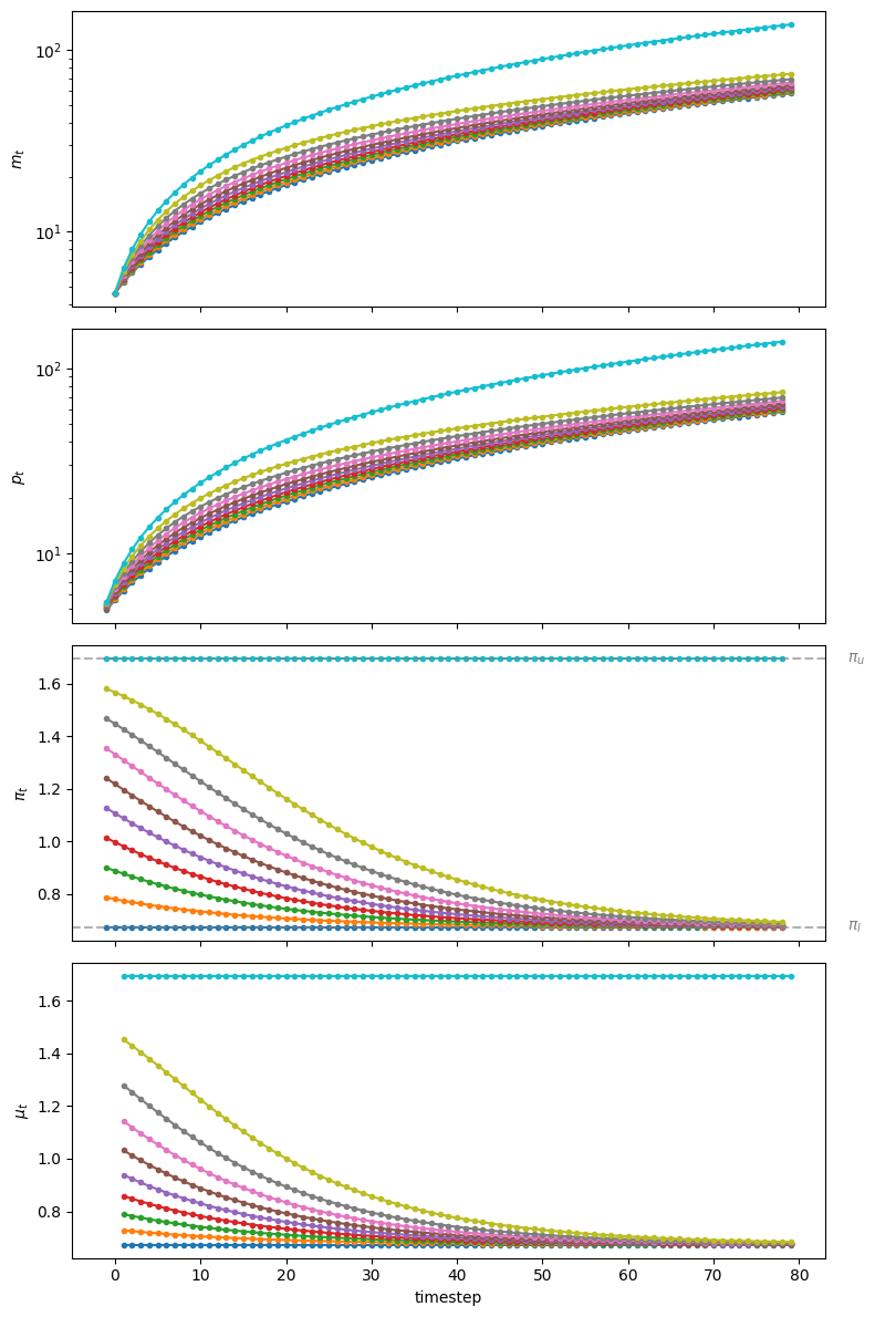
<Figure size 800x1200 with 4 Axes> — Figure 2:Starting from different initial values of $\pi_0$ , paths of $m_t$ (top panel, log scale for $m$ ), $p_t$ (second panel, log scale for $p$ ), $\pi_t$ (third panel), and $\mu_t$ (bottom panel)

References¶

Cagan, P. (1956). The Monetary Dynamics of Hyperinflation. In M. Friedman (Ed.), Studies in the Quantity Theory of Money (pp. 25–117). University of Chicago Press.
Friedman, M. (1956). A Theory of the Consumption Function. Princeton University Press.
Bruno, M., & Fischer, S. (1990). Seigniorage, operating rules, and the high inflation trap. The Quarterly Journal of Economics, 105(2), 353–374.
Marcet, A., & Sargent, T. J. (1989). Least squares learning and the dynamics of hyperinflation. In William Barnett John Geweke & K. Shell (Eds.), Sunspots, Complexity, and Chaos. Cambridge University Press.
Marcet, A., & Nicolini, J. P. (2003). Recurrent hyperinflations and learning. American Economic Review, 93(5), 1476–1498.
Sargent, T., Williams, N., & Zha, T. (2009). The conquest of South American inflation. Journal of Political Economy, 117(2), 211–256.

CC-BY-SA-4.0 — Creative Commons License – This work is licensed under a Creative Commons Attribution-ShareAlike 4.0 International.