23. Dynamics in One Dimension
23.1Overview
In economics many variables depend on their past values
For example, it seems reasonable to believe that inflation last year with affects inflation this year.
(Perhaps high inflation last year will lead people to demand higher wages to compensate, which will feed into higher prices this year.)
Letting be inflation this year and be inflation last year, we can write this relationship in a general form as
where is some function describing the relationship between the variables.
This equation is an example of one-dimensional discrete time dynamic system.
In this lecture we cover the foundations of one-dimensional discrete time dynamics.
(While most quantitative models have two or more state variables, the one-dimensional setting is a good place to learn foundations and understand key concepts.)
Let’s start with some standard imports:
import matplotlib.pyplot as plt
import numpy as np23.2Some definitions
This section sets out the objects of interest and the kinds of properties we study.
23.2.1Composition of functions
For this lecture you should know the following.
If
- is a function from to and
- is a function from to ,
then the composition of and is defined by
For example, if
- , the set of real numbers,
- and , then .
If is a function from to itself, then is the composition of with itself.
For example, if , the set of positive numbers, and , then
Similarly, if is a positive integer, then is compositions of with itself.
In the example above, .
23.2.2Dynamic systems
A (discrete time) dynamic system is a set and a function that sends set back into to itself.
Examples of dynamic systems include
- and
- and
- (the integers) and
On the other hand, if and , then and do not form a dynamic system, since .
- does not always send points in back into .
We care about dynamic systems because we can use them to study dynamics!
Given a dynamic system consisting of set and function , we can create a sequence of points in by setting
This means that we choose some number in and then take
This sequence is called the trajectory of under .
In this setting, is called the state space and is called the state variable.
Recalling that is the compositions of with itself, we can write the trajectory more simply as
In all of what follows, we are going to assume that is a subset of , the real numbers.
Equation (4) is sometimes called a first order difference equation
- first order means dependence on only one lag (i.e., earlier states such as do not enter into (4)).
23.2.3Example: a linear model
One simple example of a dynamic system is when and , where are constants (sometimes called ``parameters’').
This leads to the linear difference equation
The trajectory of is
Continuing in this way, and using our knowledge of geometric series, we find that, for any ,
We have an exact expression for for all non-negative integer and hence a full understanding of the dynamics.
Notice in particular that , then, by (9), we have
regardless of .
This is an example of what is called global stability, a topic we return to below.
23.2.4Example: a nonlinear model
In the linear example above, we obtained an exact analytical expression for in terms of arbitrary non-negative integer and .
This made analysis of dynamics very easy.
When models are nonlinear, however, the situation can be quite different.
For example, in a later lecture The Solow-Swan Growth Model, we will study the Solow-Swan growth model, which has dynamics
Here is the per capita capital stock, is the saving rate, is the total factor productivity, α is the capital share, and δ is the depreciation rate.
All these parameter are positive and .
If you try to iterate like we did in (8), you will find that the algebra gets messy quickly.
Analyzing the dynamics of this model requires a different method (see below).
23.3Stability
Consider a dynamic system consisting of set and mapping to .
23.3.1Steady states
A steady state of this system is a point in such that .
In other words, is a fixed point of the function in .
For example, for the linear model , you can use the definition to check that
- is a steady state whenever ,
- if and , then every is a steady state,
- if and , then the linear model has no steady state in .
23.3.2Global stability
A steady state of the dynamic system is called globally stable if, for all ,
For example, in the linear model with , the steady state
- is globally stable if and
- fails to be globally stable otherwise.
This follows directly from (9).
23.3.3Local stability
A steady state of the dynamic system is called locally stable if there exists an such that
Obviously every globally stable steady state is also locally stable.
Here is an example where the converse is not true.
23.4Graphical analysis
As we saw above, analyzing the dynamics for nonlinear models is nontrivial.
There is no single way to tackle all nonlinear models.
However, there is one technique for one-dimensional models that provides a great deal of intuition.
This is a graphical approach based on 45-degree diagrams.
Let’s look at an example: the Solow-Swan model with dynamics given in (11).
We begin with some plotting code that you can ignore at first reading.
The function of the code is to produce 45-degree diagrams and time series plots.
Source
def subplots():
    "Custom subplots with axes throught the origin"
    fig, ax = plt.subplots()

    # Set the axes through the origin
    for spine in ['left', 'bottom']:
        ax.spines[spine].set_position('zero')
        ax.spines[spine].set_color('green')
    for spine in ['right', 'top']:
        ax.spines[spine].set_color('none')

    return fig, ax


def plot45(g, xmin, xmax, x0, num_arrows=6, var='x'):

    xgrid = np.linspace(xmin, xmax, 200)

    fig, ax = subplots()
    ax.set_xlim(xmin, xmax)
    ax.set_ylim(xmin, xmax)
    ax.set_xlabel(r'${}_t$'.format(var), fontsize=14)
    ax.set_ylabel(r'${}_{}$'.format(var, str('{t+1}')), fontsize=14)

    hw = (xmax - xmin) * 0.01
    hl = 2 * hw
    arrow_args = dict(fc="k", ec="k", head_width=hw,
            length_includes_head=True, lw=1,
            alpha=0.6, head_length=hl)

    ax.plot(xgrid, g(xgrid), 'b-', lw=2, alpha=0.6, label='g')
    ax.plot(xgrid, xgrid, 'k-', lw=1, alpha=0.7, label='45')

    x = x0
    xticks = [xmin]
    xtick_labels = [xmin]

    for i in range(num_arrows):
        if i == 0:
            ax.arrow(x, 0.0, 0.0, g(x), **arrow_args) # x, y, dx, dy
        else:
            ax.arrow(x, x, 0.0, g(x) - x, **arrow_args)
            ax.plot((x, x), (0, x), 'k', ls='dotted')

        ax.arrow(x, g(x), g(x) - x, 0, **arrow_args)
        xticks.append(x)
        xtick_labels.append(r'${}_{}$'.format(var, str(i)))

        x = g(x)
        xticks.append(x)
        xtick_labels.append(r'${}_{}$'.format(var, str(i+1)))
        ax.plot((x, x), (0, x), 'k', ls='dotted')

    xticks.append(xmax)
    xtick_labels.append(xmax)
    ax.set_xticks(xticks)
    ax.set_yticks(xticks)
    ax.set_xticklabels(xtick_labels)
    ax.set_yticklabels(xtick_labels)

    bbox = (0., 1.04, 1., .104)
    legend_args = {'bbox_to_anchor': bbox, 'loc': 'upper right'}

    ax.legend(ncol=2, frameon=False, **legend_args, fontsize=14)
    plt.show()

def ts_plot(g, xmin, xmax, x0, ts_length=6, var='x'):
    fig, ax = subplots()
    ax.set_ylim(xmin, xmax)
    ax.set_xlabel(r'$t$', fontsize=14)
    ax.set_ylabel(r'${}_t$'.format(var), fontsize=14)
    x = np.empty(ts_length)
    x[0] = x0
    for t in range(ts_length-1):
        x[t+1] = g(x[t])
    ax.plot(range(ts_length),
            x,
            'bo-',
            alpha=0.6,
            lw=2,
            label=r'${}_t$'.format(var))
    ax.legend(loc='best', fontsize=14)
    ax.set_xticks(range(ts_length))
    plt.show()
Let’s create a 45-degree diagram for the Solow-Swan model with a fixed set of parameters. Here’s the update function corresponding to the model.
def g(k, A = 2, s = 0.3, alpha = 0.3, delta = 0.4):
    return A * s * k**alpha + (1 - delta) * k
Here is the 45-degree plot.
xmin, xmax = 0, 4  # Suitable plotting region.

plot45(g, xmin, xmax, 0, num_arrows=0)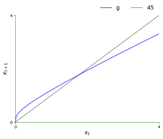
The plot shows the function and the 45-degree line.
Think of as a value on the horizontal axis.
To calculate , we can use the graph of to see its value on the vertical axis.
Clearly,
- If lies above the 45-degree line at this point, then we have .
- If lies below the 45-degree line at this point, then we have .
- If hits the 45-degree line at this point, then we have , so is a steady state.
For the Solow-Swan model, there are two steady states when .
- the origin
- the unique positive number such that .
By using some algebra, we can show that in the second case, the steady state is
23.4.1Trajectories
By the preceding discussion, in regions where lies above the 45-degree line, we know that the trajectory is increasing.
The next figure traces out a trajectory in such a region so we can see this more clearly.
The initial condition is .
k0 = 0.25

plot45(g, xmin, xmax, k0, num_arrows=5, var='k')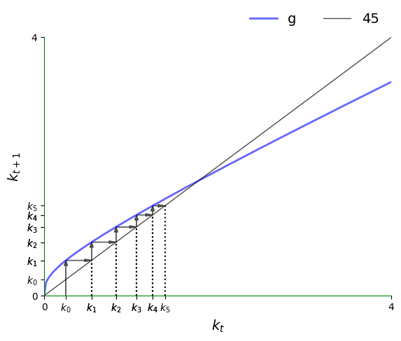
We can plot the time series of per capita capital corresponding to the figure above as follows:
ts_plot(g, xmin, xmax, k0, var='k')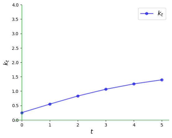
Here’s a somewhat longer view:
ts_plot(g, xmin, xmax, k0, ts_length=20, var='k')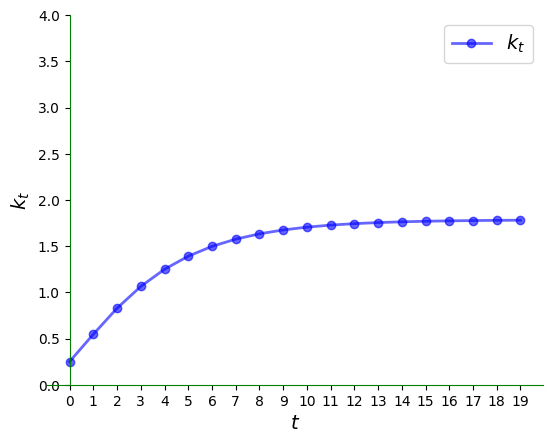
When per capita capital stock is higher than the unique positive steady state, we see that it declines:
k0 = 2.95

plot45(g, xmin, xmax, k0, num_arrows=5, var='k')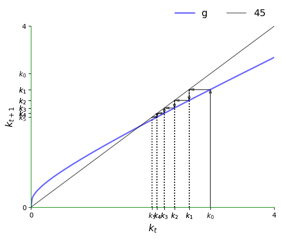
Here is the time series:
ts_plot(g, xmin, xmax, k0, var='k')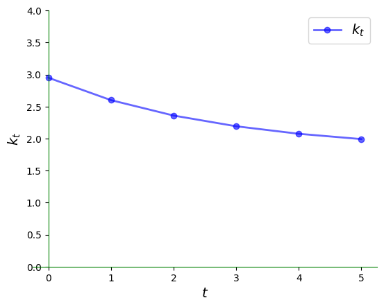
23.4.2Complex dynamics
The Solow-Swan model is nonlinear but still generates very regular dynamics.
One model that generates irregular dynamics is the quadratic map
Let’s have a look at the 45-degree diagram.
xmin, xmax = 0, 1
g = lambda x: 4 * x * (1 - x)

x0 = 0.3
plot45(g, xmin, xmax, x0, num_arrows=0)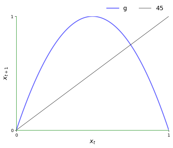
Now let’s look at a typical trajectory.
plot45(g, xmin, xmax, x0, num_arrows=6)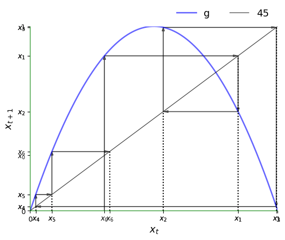
Notice how irregular it is.
Here is the corresponding time series plot.
ts_plot(g, xmin, xmax, x0, ts_length=6)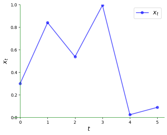
The irregularity is even clearer over a longer time horizon:
ts_plot(g, xmin, xmax, x0, ts_length=20)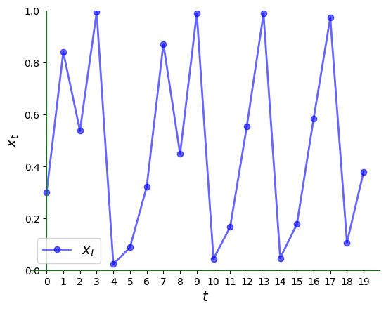
23.5Exercises
Solution to Exercise 1
We will start with the case .
Let’s set up the model and plotting region:
a, b = 0.5, 1
xmin, xmax = -1, 3
g = lambda x: a * x + b
Now let’s plot a trajectory:
x0 = -0.5
plot45(g, xmin, xmax, x0, num_arrows=5)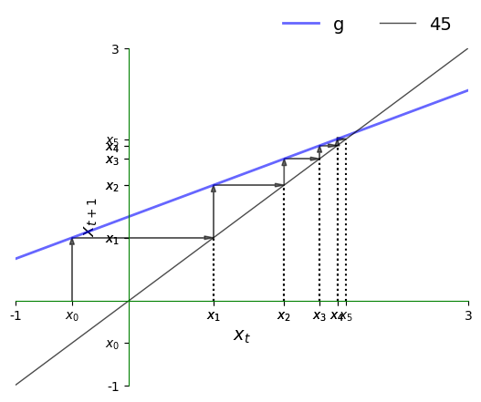
Here is the corresponding time series, which converges towards the steady state.
ts_plot(g, xmin, xmax, x0, ts_length=10)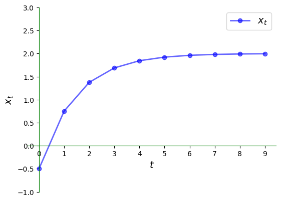
Now let’s try and see what differences we observe.
Let’s set up the model and plotting region:
a, b = -0.5, 1
xmin, xmax = -1, 3
g = lambda x: a * x + b
Now let’s plot a trajectory:
x0 = -0.5
plot45(g, xmin, xmax, x0, num_arrows=5)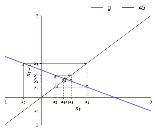
Here is the corresponding time series, which converges towards the steady state.
ts_plot(g, xmin, xmax, x0, ts_length=10)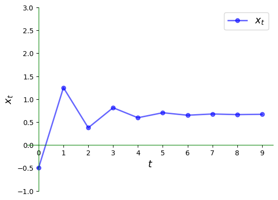
Once again, we have convergence to the steady state but the nature of convergence differs.
In particular, the time series jumps from above the steady state to below it and back again.
In the current context, the series is said to exhibit damped oscillations.

Creative Commons License – This work is licensed under a Creative Commons Attribution-ShareAlike 4.0 International.