35. Univariate Time Series with Matrix Algebra
35.1Overview
This lecture uses matrices to solve some linear difference equations.
As a running example, we’ll study a second-order linear difference equation that was the key technical tool in Paul Samuelson’s 1939 article Samuelson (1939) that introduced the multiplier-accelerator model.
This model became the workhorse that powered early econometric versions of Keynesian macroeconomic models in the United States.
You can read about the details of that model in Samuelson Multiplier-Accelerator.
(That lecture also describes some technicalities about second-order linear difference equations.)
In this lecture, we’ll also learn about an autoregressive representation and a moving average representation of a non-stationary univariate time series .
We’ll also study a “perfect foresight” model of stock prices that involves solving a “forward-looking” linear difference equation.
We will use the following imports:
import numpy as np
import matplotlib.pyplot as plt
from matplotlib import cm

# Custom figsize for this lecture
plt.rcParams["figure.figsize"] = (11, 5)

# Set decimal printing to 3 decimal places
np.set_printoptions(precision=3, suppress=True)35.2Samuelson’s model
Let index time.
For suppose that
where we assume that and are given numbers that we take as initial conditions.
In Samuelson’s model, stood for national income or perhaps a different measure of aggregate activity called gross domestic product (GDP) at time .
Equation (1) is called a second-order linear difference equation. It is called second order because it depends on two lags.
But actually, it is a collection of simultaneous linear equations in the variables .
Let’s write our equations as a stacked system
or
where
Evidently can be computed from
The vector is a complete time path .
Let’s put Python to work on an example that captures the flavor of Samuelson’s multiplier-accelerator model.
We’ll set parameters equal to the same values we used in Samuelson Multiplier-Accelerator.
T = 80

# parameters
α_0 = 10.0
α_1 = 1.53
α_2 = -.9

y_neg1 = 28.0 # y_{-1}
y_0 = 24.0
Now we construct and .
A = np.identity(T)  # The T x T identity matrix

for i in range(T):

    if i-1 >= 0:
        A[i, i-1] = -α_1

    if i-2 >= 0:
        A[i, i-2] = -α_2

b = np.full(T, α_0)
b[0] = α_0 + α_1 * y_0 + α_2 * y_neg1
b[1] = α_0 + α_2 * y_0
Let’s look at the matrix and the vector for our example.
A, b(array([[ 1. , 0. , 0. , ..., 0. , 0. , 0. ],
[-1.53, 1. , 0. , ..., 0. , 0. , 0. ],
[ 0.9 , -1.53, 1. , ..., 0. , 0. , 0. ],
...,
[ 0. , 0. , 0. , ..., 1. , 0. , 0. ],
[ 0. , 0. , 0. , ..., -1.53, 1. , 0. ],
[ 0. , 0. , 0. , ..., 0.9 , -1.53, 1. ]]),
array([ 21.52, -11.6 , 10. , 10. , 10. , 10. , 10. , 10. ,
10. , 10. , 10. , 10. , 10. , 10. , 10. , 10. ,
10. , 10. , 10. , 10. , 10. , 10. , 10. , 10. ,
10. , 10. , 10. , 10. , 10. , 10. , 10. , 10. ,
10. , 10. , 10. , 10. , 10. , 10. , 10. , 10. ,
10. , 10. , 10. , 10. , 10. , 10. , 10. , 10. ,
10. , 10. , 10. , 10. , 10. , 10. , 10. , 10. ,
10. , 10. , 10. , 10. , 10. , 10. , 10. , 10. ,
10. , 10. , 10. , 10. , 10. , 10. , 10. , 10. ,
10. , 10. , 10. , 10. , 10. , 10. , 10. , 10. ]))Now let’s solve for the path of .
If is GNP at time , then we have a version of Samuelson’s model of the dynamics for GNP.
To solve we can either invert directly, as in
A_inv = np.linalg.inv(A)

y = A_inv @ b
or we can use np.linalg.solve:
y_second_method = np.linalg.solve(A, b)Here make sure the two methods give the same result, at least up to floating point precision:
np.allclose(y, y_second_method)Trueis invertible as it is lower triangular and its diagonal entries are non-zero
# Check if A is lower triangular
np.allclose(A, np.tril(A))TrueNow we can plot.
plt.plot(np.arange(T)+1, y)
plt.xlabel('t')
plt.ylabel('y')

plt.show()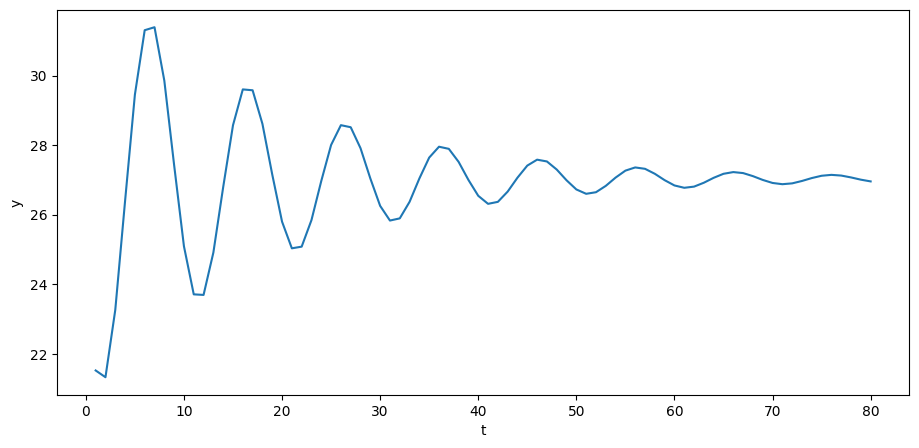
The *steady state* value of is obtained by setting in (1), which yields
If we set the initial values to , then will be constant:
y_star = α_0 / (1 - α_1 - α_2)
y_neg1_steady = y_star # y_{-1}
y_0_steady = y_star

b_steady = np.full(T, α_0)
b_steady[0] = α_0 + α_1 * y_0_steady + α_2 * y_neg1_steady
b_steady[1] = α_0 + α_2 * y_0_steady
y_steady = A_inv @ b_steadyplt.plot(np.arange(T)+1, y_steady)
plt.xlabel('t')
plt.ylabel('y')
plt.show()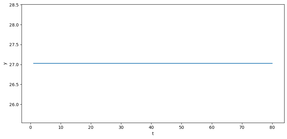
35.3Adding a random term
To generate some excitement, we’ll follow in the spirit of the great economists Eugen Slutsky and Ragnar Frisch and replace our original second-order difference equation with the following second-order stochastic linear difference equation:
where and is IID, meaning independent and identically distributed.
We’ll stack these equations into a system cast in terms of matrix algebra.
Let’s define the random vector
Where are defined as above, now assume that is governed by the system
The solution for becomes
Let’s try it out in Python.
σ_u = 2.
u = np.random.normal(0, σ_u, size=T)
y = A_inv @ (b + u)
plt.plot(np.arange(T)+1, y)
plt.xlabel('t')
plt.ylabel('y')
plt.show()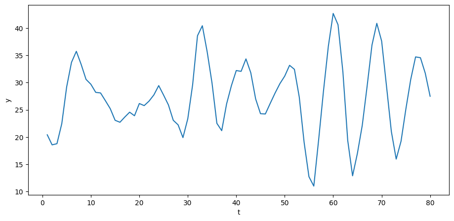
The above time series looks a lot like (detrended) GDP series for a number of advanced countries in recent decades.
We can simulate paths.
N = 100

for i in range(N):
    col = cm.viridis(np.random.rand())  # Choose a random color from viridis
    u = np.random.normal(0, σ_u, size=T)
    y = A_inv @ (b + u)
    plt.plot(np.arange(T)+1, y, lw=0.5, color=col)

plt.xlabel('t')
plt.ylabel('y')

plt.show()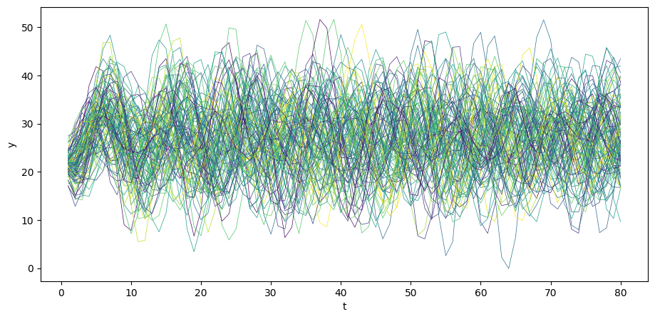
Also consider the case when and are at steady state.
N = 100

for i in range(N):
    col = cm.viridis(np.random.rand())  # Choose a random color from viridis
    u = np.random.normal(0, σ_u, size=T)
    y_steady = A_inv @ (b_steady + u)
    plt.plot(np.arange(T)+1, y_steady, lw=0.5, color=col)

plt.xlabel('t')
plt.ylabel('y')

plt.show()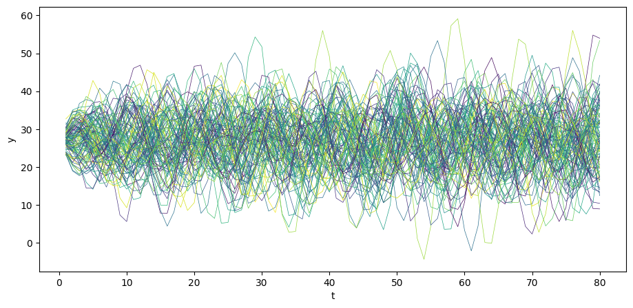
35.4Computing population moments
We can apply standard formulas for multivariate normal distributions to compute the mean vector and covariance matrix for our time series model
You can read about multivariate normal distributions in this lecture Multivariate Normal Distribution.
Let’s write our model as
where .
Because linear combinations of normal random variables are normal, we know that
where
and
Let’s write a Python class that computes the mean vector and covariance matrix .
class population_moments:
    """
    Compute population moments μ_y, Σ_y.
    ---------
    Parameters:
    α_0, α_1, α_2, T, y_neg1, y_0
    """
    def __init__(self, α_0=10.0,
                       α_1=1.53,
                       α_2=-.9,
                       T=80,
                       y_neg1=28.0,
                       y_0=24.0,
                       σ_u=1):

        # compute A
        A = np.identity(T)

        for i in range(T):
            if i-1 >= 0:
                A[i, i-1] = -α_1

            if i-2 >= 0:
                A[i, i-2] = -α_2

        # compute b
        b = np.full(T, α_0)
        b[0] = α_0 + α_1 * y_0 + α_2 * y_neg1
        b[1] = α_0 + α_2 * y_0

        # compute A inverse
        A_inv = np.linalg.inv(A)

        self.A, self.b, self.A_inv, self.σ_u, self.T = A, b, A_inv, σ_u, T

    def sample_y(self, n):
        """
        Give a sample of size n of y.
        """
        A_inv, σ_u, b, T = self.A_inv, self.σ_u, self.b, self.T
        us = np.random.normal(0, σ_u, size=[n, T])
        ys = np.vstack([A_inv @ (b + u) for u in us])

        return ys

    def get_moments(self):
        """
        Compute the population moments of y.
        """
        A_inv, σ_u, b = self.A_inv, self.σ_u, self.b

        # compute μ_y
        self.μ_y = A_inv @ b
        self.Σ_y = σ_u**2 * (A_inv @ A_inv.T)

        return self.μ_y, self.Σ_y


series_process = population_moments()

μ_y, Σ_y = series_process.get_moments()
A_inv = series_process.A_inv
It is enlightening to study the ’s implied by various parameter values.
Among other things, we can use the class to exhibit how statistical stationarity of prevails only for very special initial conditions.
Let’s begin by generating time realizations of plotting them together with population mean .
# Plot mean
N = 100

for i in range(N):
    col = cm.viridis(np.random.rand())  # Choose a random color from viridis
    ys = series_process.sample_y(N)
    plt.plot(ys[i,:], lw=0.5, color=col)
    plt.plot(μ_y, color='red')

plt.xlabel('t')
plt.ylabel('y')

plt.show()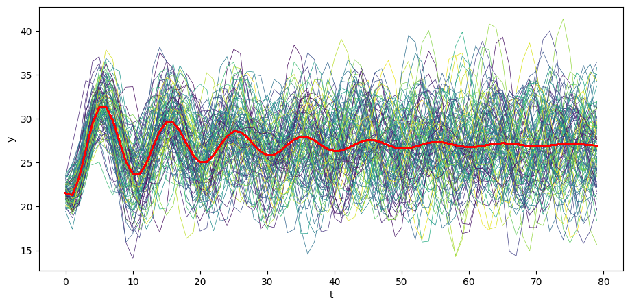
Visually, notice how the variance across realizations of decreases as increases.
Let’s plot the population variance of against .
# Plot variance
plt.plot(Σ_y.diagonal())
plt.show()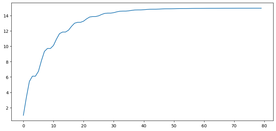
Notice how the population variance increases and asymptotes.
Let’s print out the covariance matrix for a time series .
series_process = population_moments(α_0=0,
                                    α_1=.8,
                                    α_2=0,
                                    T=6,
                                    y_neg1=0.,
                                    y_0=0.,
                                    σ_u=1)

μ_y, Σ_y = series_process.get_moments()
print("μ_y = ", μ_y)
print("Σ_y = \n", Σ_y)
μ_y = [0. 0. 0. 0. 0. 0.]
Σ_y =
[[1. 0.8 0.64 0.512 0.41 0.328]
[0.8 1.64 1.312 1.05 0.84 0.672]
[0.64 1.312 2.05 1.64 1.312 1.049]
[0.512 1.05 1.64 2.312 1.849 1.48 ]
[0.41 0.84 1.312 1.849 2.48 1.984]
[0.328 0.672 1.049 1.48 1.984 2.587]]
Notice that the covariance between and -- the elements on the superdiagonal -- are not identical.
This is an indication that the time series represented by our vector is not stationary.
To make it stationary, we’d have to alter our system so that our initial conditions are not fixed numbers but instead a jointly normally distributed random vector with a particular mean and covariance matrix.
We describe how to do that in Linear State Space Models.
But just to set the stage for that analysis, let’s print out the bottom right corner of .
series_process = population_moments()
μ_y, Σ_y = series_process.get_moments()

print("bottom right corner of Σ_y = \n", Σ_y[72:,72:])
bottom right corner of Σ_y =
[[ 14.965 12.051 4.969 -3.243 -9.434 -11.515 -9.128 -3.602]
[ 12.051 14.965 12.051 4.969 -3.243 -9.434 -11.515 -9.128]
[ 4.969 12.051 14.966 12.051 4.97 -3.243 -9.434 -11.516]
[ -3.243 4.969 12.051 14.966 12.052 4.97 -3.243 -9.434]
[ -9.434 -3.243 4.97 12.052 14.967 12.053 4.97 -3.243]
[-11.515 -9.434 -3.243 4.97 12.053 14.968 12.053 4.97 ]
[ -9.128 -11.515 -9.434 -3.243 4.97 12.053 14.968 12.053]
[ -3.602 -9.128 -11.516 -9.434 -3.243 4.97 12.053 14.968]]
Please notice how the subdiagonal and superdiagonal elements seem to have converged.
This is an indication that our process is asymptotically stationary.
You can read about stationarity of more general linear time series models in this lecture Linear State Space Models.
There is a lot to be learned about the process by staring at the off diagonal elements of corresponding to different time periods , but we resist the temptation to do so here.
35.5Moving average representation
Let’s print out and stare at its structure
- is it triangular or almost triangular or ?
To study the structure of , we shall print just up to 3 decimals.
Let’s begin by printing out just the upper left hand corner of .
print(A_inv[0:7,0:7])[[ 1. -0. -0. -0. -0. -0. -0. ]
[ 1.53 1. -0. -0. -0. -0. -0. ]
[ 1.441 1.53 1. 0. -0. 0. 0. ]
[ 0.828 1.441 1.53 1. -0. 0. 0. ]
[-0.031 0.828 1.441 1.53 1. -0. -0. ]
[-0.792 -0.031 0.828 1.441 1.53 1. 0. ]
[-1.184 -0.792 -0.031 0.828 1.441 1.53 1. ]]
Evidently, is a lower triangular matrix.
Notice how every row ends with the previous row’s pre-diagonal entries.
Since is lower triangular, each row represents for a particular as the sum of
- a time-dependent function of the initial conditions incorporated in , and
- a weighted sum of current and past values of the IID shocks .
Thus, let .
Evidently, for ,
This is a moving average representation with time-varying coefficients.
Just as system (10) constitutes a moving average representation for , system (9) constitutes an autoregressive representation for .
35.6A forward looking model
Samuelson’s model is backward looking in the sense that we give it initial conditions and let it run.
Let’s now turn to model that is forward looking.
We apply similar linear algebra machinery to study a perfect foresight model widely used as a benchmark in macroeconomics and finance.
As an example, we suppose that is the price of a stock and that is its dividend.
We assume that is determined by second-order difference equation that we analyzed just above, so that
Our perfect foresight model of stock prices is
where β is a discount factor.
The model asserts that the price of the stock at equals the discounted present values of the (perfectly foreseen) future dividends.
Form
β = .96# construct B
B = np.zeros((T, T))
for i in range(T):
B[i, i:] = β ** np.arange(0, T-i)print(B)[[1. 0.96 0.922 ... 0.043 0.041 0.04 ]
[0. 1. 0.96 ... 0.045 0.043 0.041]
[0. 0. 1. ... 0.047 0.045 0.043]
...
[0. 0. 0. ... 1. 0.96 0.922]
[0. 0. 0. ... 0. 1. 0.96 ]
[0. 0. 0. ... 0. 0. 1. ]]
σ_u = 0.
u = np.random.normal(0, σ_u, size=T)
y = A_inv @ (b + u)
y_steady = A_inv @ (b_steady + u)
p = B @ yplt.plot(np.arange(0, T)+1, y, label='y')
plt.plot(np.arange(0, T)+1, p, label='p')
plt.xlabel('t')
plt.ylabel('y/p')
plt.legend()
plt.show()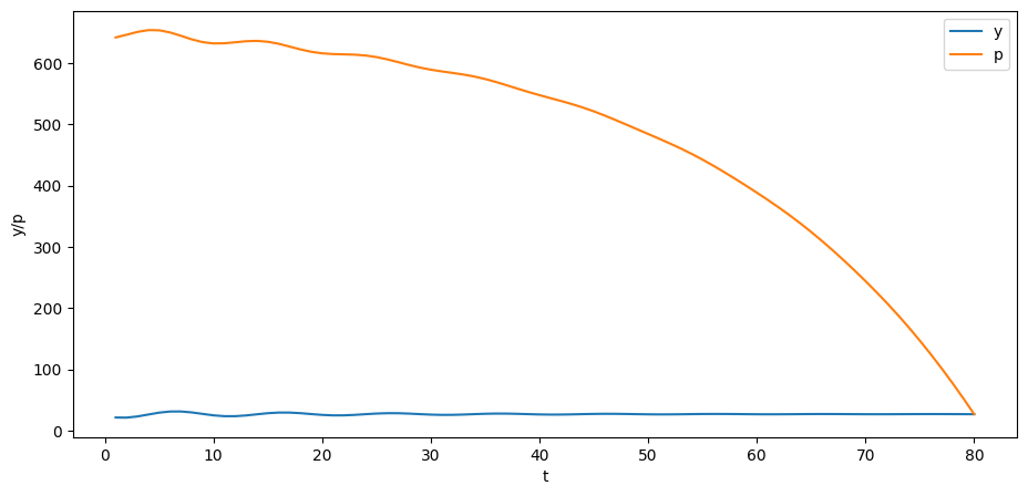
Can you explain why the trend of the price is downward over time?
Also consider the case when and are at the steady state.
p_steady = B @ y_steady

plt.plot(np.arange(0, T)+1, y_steady, label='y')
plt.plot(np.arange(0, T)+1, p_steady, label='p')
plt.xlabel('t')
plt.ylabel('y/p')
plt.legend()

plt.show()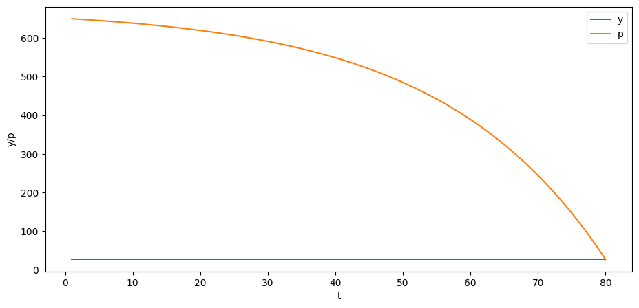
- Samuelson, P. A. (1939). Interactions Between the Multiplier Analysis and the Principle of Acceleration. Review of Economic Studies, 21(2), 75–78.

Creative Commons License – This work is licensed under a Creative Commons Attribution-ShareAlike 4.0 International.