37. Shortest Paths

37.1Overview¶

The shortest path problem is a classic problem in mathematics and computer science with applications in

• Economics (sequential decision making, analysis of social networks, etc.)
• Operations research and transportation
• Robotics and artificial intelligence
• Telecommunication network design and routing
• etc., etc.

Variations of the methods we discuss in this lecture are used millions of times every day, in applications such as

• Google Maps
• routing packets on the internet

For us, the shortest path problem also provides a nice introduction to the logic of dynamic programming.

Dynamic programming is an extremely powerful optimization technique that we apply in many lectures on this site.

The only scientific library we’ll need in what follows is NumPy:

37.2Outline of the problem¶

The shortest path problem is one of finding how to traverse a graph from one specified node to another at minimum cost.

Consider the following graph

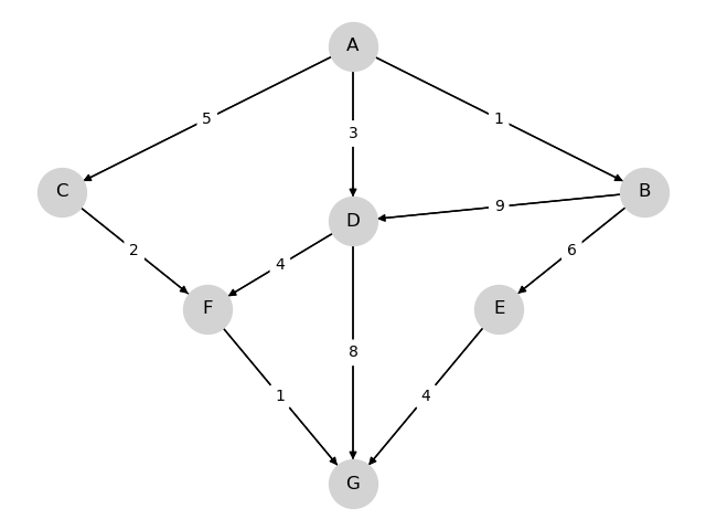
We wish to travel from node (vertex) A to node G at minimum cost

• Arrows (edges) indicate the movements we can take.
• Numbers on edges indicate the cost of traveling that edge.

(Graphs such as the one above are called weighted directed graphs.)

Possible interpretations of the graph include

• Minimum cost for supplier to reach a destination.
• Routing of packets on the internet (minimize time).
• etc., etc.

For this simple graph, a quick scan of the edges shows that the optimal paths are

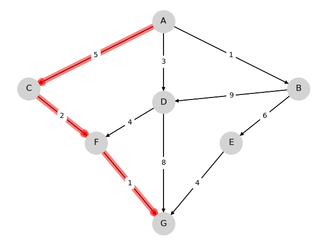
• A, C, F, G at cost 8

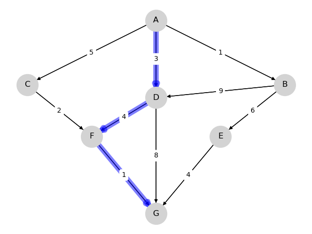
• A, D, F, G at cost 8

37.3Finding least-cost paths¶

For large graphs, we need a systematic solution.

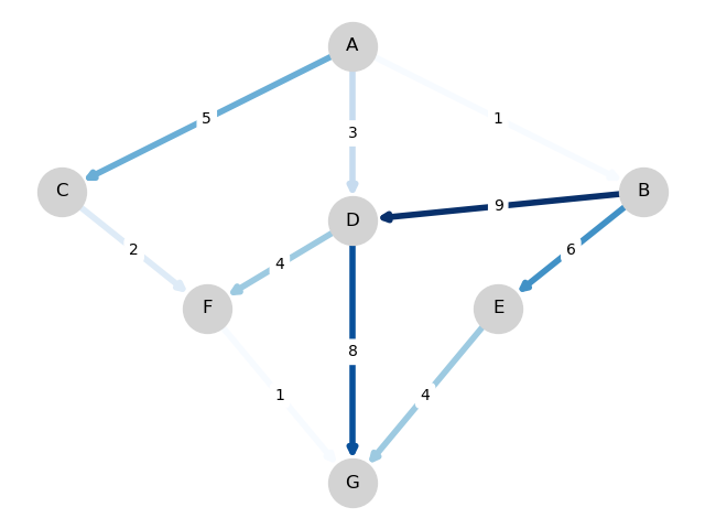
Let $J(v)$ denote the minimum cost-to-go from node $v$, understood as the total cost from $v$ if we take the best route.

Suppose that we know $J(v)$ for each node $v$, as shown below for the graph from the preceding example.

Note that $J(G) = 0$.

The best path can now be found as follows

1. Start at node $v = A$
2. From current node $v$, move to any node that solves

where

• $F_v$ is the set of nodes that can be reached from $v$ in one step.
• $c(v, w)$ is the cost of traveling from $v$ to $w$.

Hence, if we know the function $J$, then finding the best path is almost trivial.

But how can we find the cost-to-go function $J$?

Some thought will convince you that, for every node $v$, the function $J$ satisfies

This is known as the Bellman equation, after the mathematician Richard Bellman.

The Bellman equation can be thought of as a restriction that $J$ must satisfy.

What we want to do now is use this restriction to compute $J$.

37.4Solving for minimum cost-to-go¶

Let’s look at an algorithm for computing $J$ and then think about how to implement it.

37.4.1The algorithm¶

The standard algorithm for finding $J$ is to start an initial guess and then iterate.

This is a standard approach to solving nonlinear equations, often called the method of successive approximations.

Our initial guess will be

Now

1. Set $n = 0$
2. Set $J_{n+1} (v) = \min_{w \in F_v} \{ c(v, w) + J_n(w) \}$ for all $v$
3. If $J_{n+1}$ and $J_n$ are not equal then increment $n$, go to 2

This sequence converges to $J$.

Although we omit the proof, we’ll prove similar claims in our other lectures on dynamic programming.

37.4.2Implementation¶

Having an algorithm is a good start, but we also need to think about how to implement it on a computer.

First, for the cost function $c$, we’ll implement it as a matrix $Q$, where a typical element is

In this context $Q$ is usually called the distance matrix.

We’re also numbering the nodes now, with $A = 0$, so, for example

For example, for the simple graph above, we set

Notice that the cost of staying still (on the principle diagonal) is set to

• np.inf for non-destination nodes --- moving on is required.
• 0 for the destination node --- here is where we stop.

For the sequence of approximations $\{J_n\}$ of the cost-to-go functions, we can use NumPy arrays.

Let’s try with this example and see how we go:

This matches with the numbers we obtained by inspection above.

But, importantly, we now have a methodology for tackling large graphs.

37.5Exercises¶

num_nodes = 100
destination_node = 99

def map_graph_to_distance_matrix(in_file):

    # First let's set of the distance matrix Q with inf everywhere
    Q = np.full((num_nodes, num_nodes), np.inf)

    # Now we read in the data and modify Q
    with open(in_file) as infile:
        for line in infile:
            elements = line.split(',')
            node = elements.pop(0)
            node = int(node[4:])    # convert node description to integer
            if node != destination_node:
                for element in elements:
                    destination, cost = element.split()
                    destination = int(destination[4:])
                    Q[node, destination] = float(cost)
            Q[destination_node, destination_node] = 0
    return Q

def bellman(J, Q):
    return np.min(Q + J, axis=1)


def compute_cost_to_go(Q):
    num_nodes = Q.shape[0]
    J = np.zeros(num_nodes)      # Initial guess
    max_iter = 500
    i = 0

    while i < max_iter:
        next_J = bellman(J, Q)
        if np.allclose(next_J, J):
            break
        else:
            J[:] = next_J   # Copy contents of next_J to J
            i += 1

    return(J)

def print_best_path(J, Q):
    sum_costs = 0
    current_node = 0
    while current_node != destination_node:
        print(current_node)
        # Move to the next node and increment costs
        next_node = np.argmin(Q[current_node, :] + J)
        sum_costs += Q[current_node, next_node]
        current_node = next_node

    print(destination_node)
    print('Cost: ', sum_costs)

Q = map_graph_to_distance_matrix('graph.txt')
J = compute_cost_to_go(Q)
print_best_path(J, Q)

0
8
11
18
23
33
41
53
56
57
60
67
70
73
76
85
87
88
93
94
96
97
98
99
Cost:  160.55000000000007

J[0]