8. Linear Equations and Matrix Algebra

8.1Overview¶

Many problems in economics and finance require solving linear equations.

In this lecture we discuss linear equations and their applications.

To illustrate the importance of linear equations, we begin with a two good model of supply and demand.

The two good case is so simple that solutions can be calculated by hand.

But often we need to consider markets containing many goods.

In the multiple goods case we face large systems of linear equations, with many equations and unknowns.

To handle such systems we need two things:

• matrix algebra (and the knowledge of how to use it) plus
• computer code to apply matrix algebra to the problems of interest.

This lecture covers these steps.

We will use the following packages:

8.2A two good example¶

In this section we discuss a simple two good example and solve it by

1. pencil and paper
2. matrix algebra

The second method is more general, as we will see.

8.2.1Pencil and paper methods¶

Suppose that we have two related goods, such as

• propane and ethanol, and
• rice and wheat, etc.

To keep things simple, we label them as good 0 and good 1.

The demand for each good depends on the price of both goods:

(We are assuming demand decreases when the price of either good goes up, but other cases are also possible.)

Let’s suppose that supply is given by

Equilibrium holds when supply equals demand ($q_0^s = q_0^d$ and $q_1^s = q_1^d$).

This yields the linear system

We can solve this with pencil and paper to get

Inserting these results into either (1) or (2) yields the equilibrium quantities

8.2.2Looking forward¶

Pencil and paper methods are easy in the two good case.

But what if there are many goods?

For such problems we need matrix algebra.

Before solving problems with matrix algebra, let’s first recall the basics of vectors and matrices, in both theory and computation.

8.3Vectors ¶

A vector of length $n$ is just a sequence (or array, or tuple) of $n$ numbers, which we write as $x = (x_1, \ldots, x_n)$ or $x = \begin{bmatrix}x_1, \ldots, x_n\end{bmatrix}$.

We can write these sequences either horizontally or vertically.

But when we use matrix operations, our default assumption is that vectors are column vectors.

The set of all $n$-vectors is denoted by $\mathbb R^n$.

Often vectors are represented visually as arrows from the origin to the point.

Here’s a visualization.

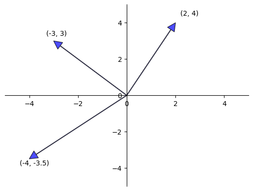
8.3.1Vector operations¶

Sometimes we want to modify vectors.

The two most common operators on vectors are addition and scalar multiplication, which we now describe.

When we add two vectors, we add them element-by-element.

In general,

We can visualise vector addition in $\mathbb{R}^2$ as follows.

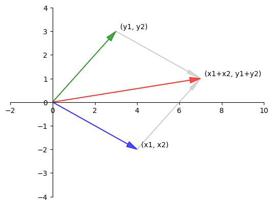
Scalar multiplication is an operation that multiplies a vector $x$ with a scalar elementwise.

More generally, it takes a number γ and a vector $x$ and produces

Scalar multiplication is illustrated in the next figure.

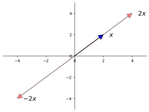
In Python, a vector can be represented as a list or tuple, such as x = [2, 4, 6] or x = (2, 4, 6).

However, it is more common to represent vectors with NumPy arrays.

One advantage of NumPy arrays is that scalar multiplication and addition have very natural syntax.

8.3.2Inner product and norm¶

The inner product of vectors $x,y \in \mathbb R^n$ is defined as

The norm of a vector $x$ represents its “length” (i.e., its distance from the zero vector) and is defined as

The expression $\| x - y\|$ can be thought of as the “distance” between $x$ and $y$.

The inner product and norm can be computed as follows

8.4Matrix operations¶

When we discussed linear price systems, we mentioned using matrix algebra.

Matrix algebra is similar to algebra for numbers.

Let’s review some details.

8.4.1Addition and scalar multiplication¶

Just as was the case for vectors, we can add, subtract and scalar multiply matrices.

Scalar multiplication and addition are generalizations of the vector case:

In general for a number γ and any matrix $A$,

In general,

In the latter case, the matrices must have the same shape in order for the definition to make sense.

8.4.2Matrix multiplication¶

We also have a convention for multiplying two matrices.

The rule for matrix multiplication generalizes the idea of inner products discussed above.

If $A$ and $B$ are two matrices, then their product $A B$ is formed by taking as its $i,j$-th element the inner product of the $i$-th row of $A$ and the $j$-th column of $B$.

If $A$ is $n \times k$ and $B$ is $j \times m$, then to multiply $A$ and $B$ we require $k = j$, and the resulting matrix $A B$ is $n \times m$.

As an important special case, consider multiplying $n \times k$ matrix $A$ and $k \times 1$ column vector $x$.

According to the preceding rule, this gives us an $n \times 1$ column vector.

Here is a simple illustration of multiplication of two matrices.

There are many tutorials to help you further visualize this operation, such as

• this one, or
• the discussion on the Wikipedia page.

One important special case is the identity matrix, which has ones on the principal diagonal and zero elsewhere:

It is a useful exercise to check the following:

• if $A$ is $n \times k$ and $I$ is the $k \times k$ identity matrix, then $AI = A$, and
• if $I$ is the $n \times n$ identity matrix, then $IA = A$.

8.4.3Matrices in NumPy¶

NumPy arrays are also used as matrices, and have fast, efficient functions and methods for all the standard matrix operations.

You can create them manually from tuples of tuples (or lists of lists) as follows

The shape attribute is a tuple giving the number of rows and columns --- see here for more discussion.

To get the transpose of A, use A.transpose() or, more simply, A.T.

There are many convenient functions for creating common matrices (matrices of zeros, ones, etc.) --- see here.

Since operations are performed elementwise by default, scalar multiplication and addition have very natural syntax.

To multiply matrices we use the @ symbol.

8.4.4Two good model in matrix form¶

We can now revisit the two good model and solve (3) numerically via matrix algebra.

This involves some extra steps but the method is widely applicable --- as we will see when we include more goods.

First we rewrite (1) as

Recall that $p \in \mathbb{R}^{2}$ is the price of two goods.

(Please check that $q^d = D p + h$ represents the same equations as (1).)

We rewrite (2) as

Now equality of supply and demand can be expressed as $q^s = q^d$, or

We can rearrange the terms to get

If all of the terms were numbers, we could solve for prices as $p = h / (C-D)$.

Matrix algebra allows us to do something similar: we can solve for equilibrium prices using the inverse of $C - D$:

Before we implement the solution let us consider a more general setting.

8.4.5More goods¶

It is natural to think about demand systems with more goods.

For example, even within energy commodities there are many different goods, including crude oil, gasoline, coal, natural gas, ethanol, and uranium.

The prices of these goods are related, so it makes sense to study them together.

Pencil and paper methods become very time consuming with large systems.

But fortunately the matrix methods described above are essentially unchanged.

In general, we can write the demand equation as $q^d = Dp + h$, where

• $q^d$ is an $n \times 1$ vector of demand quantities for $n$ different goods.
• $D$ is an $n \times n$ “coefficient” matrix.
• $h$ is an $n \times 1$ vector of constant values.

Similarly, we can write the supply equation as $q^s = Cp + e$, where

• $q^s$ is an $n \times 1$ vector of supply quantities for the same goods.
• $C$ is an $n \times n$ “coefficient” matrix.
• $e$ is an $n \times 1$ vector of constant values.

To find an equilibrium, we solve $Dp + h = Cp + e$, or

Then the price vector of the n different goods is

8.4.6General linear systems¶

A more general version of the problem described above looks as follows.

The objective here is to solve for the “unknowns” $x_1, \ldots, x_n$.

We take as given the coefficients $a_{11}, \ldots, a_{nn}$ and constants $b_1, \ldots, b_n$.

Notice that we are treating a setting where the number of unknowns equals the number of equations.

This is the case where we are most likely to find a well-defined solution.

(The other cases are referred to as overdetermined and underdetermined systems of equations --- we defer discussion of these cases until later lectures.)

In matrix form, the system (27) becomes

When considering problems such as (28), we need to ask at least some of the following questions

• Does a solution actually exist?
• If a solution exists, how should we compute it?

8.5Solving systems of equations¶

Recall again the system of equations (27), which we write here again as

The problem we face is to find a vector $x \in \mathbb R^n$ that solves (30), taking $b$ and $A$ as given.

We may not always find a unique vector $x$ that solves (30).

We illustrate two such cases below.

8.5.1No solution¶

Consider the system of equations given by,

It can be verified manually that this system has no possible solution.

To illustrate why this situation arises let’s plot the two lines.

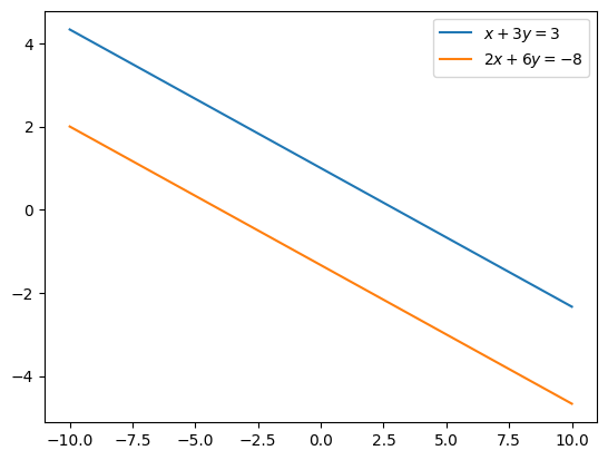
Clearly, these are parallel lines and hence we will never find a point $x \in \mathbb{R}^2$ such that these lines intersect.

Thus, this system has no possible solution.

We can rewrite this system in matrix form as

It can be noted that the $2^{nd}$ row of matrix $A = (2, 6)$ is just a scalar multiple of the $1^{st}$ row of matrix $A = (1, 3)$.

The rows of matrix $A$ in this case are called linearly dependent.

8.5.2Many solutions¶

Now consider,

Any vector $v = (x,y)$ such that $x = 2y - 4$ will solve the above system.

Since we can find infinite such vectors this system has infinitely many solutions.

This is because the rows of the corresponding matrix

are linearly dependent --- can you see why?

We now impose conditions on $A$ in (30) that rule out these problems.

8.5.3Nonsingular matrices¶

To every square matrix we can assign a unique number called the determinant.

For $2 \times 2$ matrices, the determinant is given by,

If the determinant of $A$ is not zero, then we say that $A$ is nonsingular.

A square matrix $A$ is nonsingular if and only if the rows and columns of $A$ are linearly independent.

A more detailed explanation of matrix inverse can be found here.

You can check yourself that the in (32) and (34) with linearly dependent rows are singular matrices.

This gives us a useful one-number summary of whether or not a square matrix can be inverted.

In particular, a square matrix $A$ has a nonzero determinant, if and only if it possesses an inverse matrix $A^{-1}$, with the property that $A A^{-1} = A^{-1} A = I$.

As a consequence, if we pre-multiply both sides of $Ax = b$ by $A^{-1}$, we get

This is the solution to $Ax = b$ --- the solution we are looking for.

8.5.4Linear equations with NumPy¶

In the two good example we obtained the matrix equation,

where $C$, $D$ and $h$ are given by (20) and (21).

This equation is analogous to (36) with $A = (C-D)^{-1}$, $b = h$, and $x = p$.

We can now solve for equilibrium prices with NumPy’s linalg submodule.

All of these routines are Python front ends to time-tested and highly optimized FORTRAN code.

Now we change this to a NumPy array.

Notice that we get the same solutions as the pencil and paper case.

We can also solve for $p$ using solve(A, h) as follows.

Observe how we can solve for $x = A^{-1} y$ by either via inv(A) @ y, or using solve(A, y).

The latter method uses a different algorithm that is numerically more stable and hence should be the default option.

8.6Exercises¶

import numpy as np
from numpy.linalg import det

A = np.array([[35, -5, -5],  # matrix A
              [-5, 25, -10],
              [-5, -5, 15]])

b = np.array((100, 75, 55))  # column vector b
b.shape = (3, 1)

det(A)  # check if A is nonsingular

# Using inverse
from numpy.linalg import det

A_inv = inv(A)

p = A_inv @ b
p

# Using numpy.linalg.solve
from numpy.linalg import solve
p = solve(A, b)
p

Solution to Exercise 2

import numpy as np
from numpy.linalg import inv

# Using matrix algebra
A = np.array([[1, -9],  # matrix A
              [1, -7],
              [1, -3]])

A_T = np.transpose(A)  # transpose of matrix A

b = np.array((1, 3, 8))  # column vector b
b.shape = (3, 1)

x = inv(A_T @ A) @ A_T @ b
x

array([[11.46428571], [ 1.17857143]])

# Using numpy.linalg.lstsq
x, res, _, _ = np.linalg.lstsq(A, b, rcond=None)

Source

print(f"x\u0302 = {x}")
print(f"\u2016Ax\u0302 - b\u2016\u00B2 = {res[0]}")

x̂ = [[11.46428571]
 [ 1.17857143]]
‖Ax̂ - b‖² = 0.07142857142857066

Here is a visualization of how the least squares method approximates the equation of a line connecting a set of points.

We can also describe this as “fitting” a line between a set of points.

fig, ax = plt.subplots()
p = np.array((1, 3, 8))
q = np.array((9, 7, 3))

a, b = x

ax.plot(q, p, 'o', label='observations', markersize=5)
ax.plot(q, a - b*q, 'r', label='Fitted line')
plt.xlabel('quantity demanded')
plt.ylabel('price')
plt.legend()
plt.show()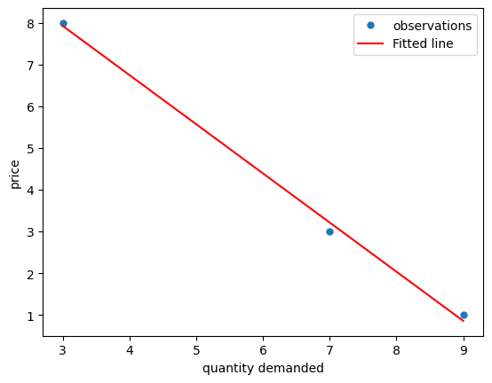

8.6.1Further reading¶

The documentation of the numpy.linalg submodule can be found here.

More advanced topics in linear algebra can be found here.