Input-Output Models - A First Course in Quantitative Economics with Python

A First Course in Quantitative Economics with Python

Input-Output Models

and

39.1Overview¶

This lecture requires the following imports and installs before we proceed.

!pip install quantecon_book_networks
!pip install quantecon
!pip install pandas-datareader

Output

Collecting quantecon_book_networks
  Using cached quantecon_book_networks-1.1-py2.py3-none-any.whl.metadata (1.3 kB)

Requirement already satisfied: numpy in /opt/hostedtoolcache/Python/3.12.9/x64/lib/python3.12/site-packages (from quantecon_book_networks) (2.1.3)
Requirement already satisfied: scipy in /opt/hostedtoolcache/Python/3.12.9/x64/lib/python3.12/site-packages (from quantecon_book_networks) (1.15.2)
Requirement already satisfied: pandas in /opt/hostedtoolcache/Python/3.12.9/x64/lib/python3.12/site-packages (from quantecon_book_networks) (2.2.3)
Requirement already satisfied: matplotlib in /opt/hostedtoolcache/Python/3.12.9/x64/lib/python3.12/site-packages (from quantecon_book_networks) (3.10.0)

Collecting pandas-datareader (from quantecon_book_networks)
  Using cached pandas_datareader-0.10.0-py3-none-any.whl.metadata (2.9 kB)

Requirement already satisfied: networkx in /opt/hostedtoolcache/Python/3.12.9/x64/lib/python3.12/site-packages (from quantecon_book_networks) (3.4.2)
Requirement already satisfied: quantecon in /opt/hostedtoolcache/Python/3.12.9/x64/lib/python3.12/site-packages (from quantecon_book_networks) (0.8.0)

Collecting POT (from quantecon_book_networks)

  Using cached POT-0.9.5-cp312-cp312-manylinux_2_17_x86_64.manylinux2014_x86_64.whl.metadata (34 kB)

Requirement already satisfied: contourpy>=1.0.1 in /opt/hostedtoolcache/Python/3.12.9/x64/lib/python3.12/site-packages (from matplotlib->quantecon_book_networks) (1.3.1)

Requirement already satisfied: cycler>=0.10 in /opt/hostedtoolcache/Python/3.12.9/x64/lib/python3.12/site-packages (from matplotlib->quantecon_book_networks) (0.12.1)
Requirement already satisfied: fonttools>=4.22.0 in /opt/hostedtoolcache/Python/3.12.9/x64/lib/python3.12/site-packages (from matplotlib->quantecon_book_networks) (4.56.0)
Requirement already satisfied: kiwisolver>=1.3.1 in /opt/hostedtoolcache/Python/3.12.9/x64/lib/python3.12/site-packages (from matplotlib->quantecon_book_networks) (1.4.8)
Requirement already satisfied: packaging>=20.0 in /opt/hostedtoolcache/Python/3.12.9/x64/lib/python3.12/site-packages (from matplotlib->quantecon_book_networks) (24.2)
Requirement already satisfied: pillow>=8 in /opt/hostedtoolcache/Python/3.12.9/x64/lib/python3.12/site-packages (from matplotlib->quantecon_book_networks) (11.1.0)

Requirement already satisfied: pyparsing>=2.3.1 in /opt/hostedtoolcache/Python/3.12.9/x64/lib/python3.12/site-packages (from matplotlib->quantecon_book_networks) (3.2.1)
Requirement already satisfied: python-dateutil>=2.7 in /opt/hostedtoolcache/Python/3.12.9/x64/lib/python3.12/site-packages (from matplotlib->quantecon_book_networks) (2.9.0.post0)

Requirement already satisfied: pytz>=2020.1 in /opt/hostedtoolcache/Python/3.12.9/x64/lib/python3.12/site-packages (from pandas->quantecon_book_networks) (2025.1)
Requirement already satisfied: tzdata>=2022.7 in /opt/hostedtoolcache/Python/3.12.9/x64/lib/python3.12/site-packages (from pandas->quantecon_book_networks) (2025.1)

Collecting lxml (from pandas-datareader->quantecon_book_networks)
  Using cached lxml-5.3.1-cp312-cp312-manylinux_2_28_x86_64.whl.metadata (3.7 kB)


Requirement already satisfied: requests>=2.19.0 in /opt/hostedtoolcache/Python/3.12.9/x64/lib/python3.12/site-packages (from pandas-datareader->quantecon_book_networks) (2.32.3)

Requirement already satisfied: numba>=0.49.0 in /opt/hostedtoolcache/Python/3.12.9/x64/lib/python3.12/site-packages (from quantecon->quantecon_book_networks) (0.61.0)

Requirement already satisfied: sympy in /opt/hostedtoolcache/Python/3.12.9/x64/lib/python3.12/site-packages (from quantecon->quantecon_book_networks) (1.13.3)

Requirement already satisfied: llvmlite<0.45,>=0.44.0dev0 in /opt/hostedtoolcache/Python/3.12.9/x64/lib/python3.12/site-packages (from numba>=0.49.0->quantecon->quantecon_book_networks) (0.44.0)

Requirement already satisfied: six>=1.5 in /opt/hostedtoolcache/Python/3.12.9/x64/lib/python3.12/site-packages (from python-dateutil>=2.7->matplotlib->quantecon_book_networks) (1.17.0)

Requirement already satisfied: charset-normalizer<4,>=2 in /opt/hostedtoolcache/Python/3.12.9/x64/lib/python3.12/site-packages (from requests>=2.19.0->pandas-datareader->quantecon_book_networks) (3.4.1)


Requirement already satisfied: idna<4,>=2.5 in /opt/hostedtoolcache/Python/3.12.9/x64/lib/python3.12/site-packages (from requests>=2.19.0->pandas-datareader->quantecon_book_networks) (3.10)
Requirement already satisfied: urllib3<3,>=1.21.1 in /opt/hostedtoolcache/Python/3.12.9/x64/lib/python3.12/site-packages (from requests>=2.19.0->pandas-datareader->quantecon_book_networks) (2.3.0)
Requirement already satisfied: certifi>=2017.4.17 in /opt/hostedtoolcache/Python/3.12.9/x64/lib/python3.12/site-packages (from requests>=2.19.0->pandas-datareader->quantecon_book_networks) (2025.1.31)

Requirement already satisfied: mpmath<1.4,>=1.1.0 in /opt/hostedtoolcache/Python/3.12.9/x64/lib/python3.12/site-packages (from sympy->quantecon->quantecon_book_networks) (1.3.0)

Using cached quantecon_book_networks-1.1-py2.py3-none-any.whl (364 kB)
Using cached pandas_datareader-0.10.0-py3-none-any.whl (109 kB)
Using cached POT-0.9.5-cp312-cp312-manylinux_2_17_x86_64.manylinux2014_x86_64.whl (901 kB)


Using cached lxml-5.3.1-cp312-cp312-manylinux_2_28_x86_64.whl (5.0 MB)

Installing collected packages: lxml, POT, pandas-datareader, quantecon_book_networks

Successfully installed POT-0.9.5 lxml-5.3.1 pandas-datareader-0.10.0 quantecon_book_networks-1.1

Requirement already satisfied: quantecon in /opt/hostedtoolcache/Python/3.12.9/x64/lib/python3.12/site-packages (0.8.0)

Requirement already satisfied: numba>=0.49.0 in /opt/hostedtoolcache/Python/3.12.9/x64/lib/python3.12/site-packages (from quantecon) (0.61.0)
Requirement already satisfied: numpy>=1.17.0 in /opt/hostedtoolcache/Python/3.12.9/x64/lib/python3.12/site-packages (from quantecon) (2.1.3)
Requirement already satisfied: requests in /opt/hostedtoolcache/Python/3.12.9/x64/lib/python3.12/site-packages (from quantecon) (2.32.3)
Requirement already satisfied: scipy>=1.5.0 in /opt/hostedtoolcache/Python/3.12.9/x64/lib/python3.12/site-packages (from quantecon) (1.15.2)
Requirement already satisfied: sympy in /opt/hostedtoolcache/Python/3.12.9/x64/lib/python3.12/site-packages (from quantecon) (1.13.3)

Requirement already satisfied: llvmlite<0.45,>=0.44.0dev0 in /opt/hostedtoolcache/Python/3.12.9/x64/lib/python3.12/site-packages (from numba>=0.49.0->quantecon) (0.44.0)

Requirement already satisfied: charset-normalizer<4,>=2 in /opt/hostedtoolcache/Python/3.12.9/x64/lib/python3.12/site-packages (from requests->quantecon) (3.4.1)
Requirement already satisfied: idna<4,>=2.5 in /opt/hostedtoolcache/Python/3.12.9/x64/lib/python3.12/site-packages (from requests->quantecon) (3.10)

Requirement already satisfied: urllib3<3,>=1.21.1 in /opt/hostedtoolcache/Python/3.12.9/x64/lib/python3.12/site-packages (from requests->quantecon) (2.3.0)
Requirement already satisfied: certifi>=2017.4.17 in /opt/hostedtoolcache/Python/3.12.9/x64/lib/python3.12/site-packages (from requests->quantecon) (2025.1.31)
Requirement already satisfied: mpmath<1.4,>=1.1.0 in /opt/hostedtoolcache/Python/3.12.9/x64/lib/python3.12/site-packages (from sympy->quantecon) (1.3.0)

Requirement already satisfied: pandas-datareader in /opt/hostedtoolcache/Python/3.12.9/x64/lib/python3.12/site-packages (0.10.0)
Requirement already satisfied: lxml in /opt/hostedtoolcache/Python/3.12.9/x64/lib/python3.12/site-packages (from pandas-datareader) (5.3.1)
Requirement already satisfied: pandas>=0.23 in /opt/hostedtoolcache/Python/3.12.9/x64/lib/python3.12/site-packages (from pandas-datareader) (2.2.3)
Requirement already satisfied: requests>=2.19.0 in /opt/hostedtoolcache/Python/3.12.9/x64/lib/python3.12/site-packages (from pandas-datareader) (2.32.3)

Requirement already satisfied: numpy>=1.26.0 in /opt/hostedtoolcache/Python/3.12.9/x64/lib/python3.12/site-packages (from pandas>=0.23->pandas-datareader) (2.1.3)
Requirement already satisfied: python-dateutil>=2.8.2 in /opt/hostedtoolcache/Python/3.12.9/x64/lib/python3.12/site-packages (from pandas>=0.23->pandas-datareader) (2.9.0.post0)
Requirement already satisfied: pytz>=2020.1 in /opt/hostedtoolcache/Python/3.12.9/x64/lib/python3.12/site-packages (from pandas>=0.23->pandas-datareader) (2025.1)
Requirement already satisfied: tzdata>=2022.7 in /opt/hostedtoolcache/Python/3.12.9/x64/lib/python3.12/site-packages (from pandas>=0.23->pandas-datareader) (2025.1)
Requirement already satisfied: charset-normalizer<4,>=2 in /opt/hostedtoolcache/Python/3.12.9/x64/lib/python3.12/site-packages (from requests>=2.19.0->pandas-datareader) (3.4.1)

Requirement already satisfied: idna<4,>=2.5 in /opt/hostedtoolcache/Python/3.12.9/x64/lib/python3.12/site-packages (from requests>=2.19.0->pandas-datareader) (3.10)
Requirement already satisfied: urllib3<3,>=1.21.1 in /opt/hostedtoolcache/Python/3.12.9/x64/lib/python3.12/site-packages (from requests>=2.19.0->pandas-datareader) (2.3.0)
Requirement already satisfied: certifi>=2017.4.17 in /opt/hostedtoolcache/Python/3.12.9/x64/lib/python3.12/site-packages (from requests>=2.19.0->pandas-datareader) (2025.1.31)

Requirement already satisfied: six>=1.5 in /opt/hostedtoolcache/Python/3.12.9/x64/lib/python3.12/site-packages (from python-dateutil>=2.8.2->pandas>=0.23->pandas-datareader) (1.17.0)

import numpy as np
import networkx as nx
import matplotlib.pyplot as plt
import quantecon_book_networks
import quantecon_book_networks.input_output as qbn_io
import quantecon_book_networks.plotting as qbn_plt
import quantecon_book_networks.data as qbn_data
import matplotlib as mpl
from matplotlib.patches import Polygon

quantecon_book_networks.config("matplotlib")
mpl.rcParams.update(mpl.rcParamsDefault)

The following figure illustrates a network of linkages among 15 sectors obtained from the US Bureau of Economic Analysis’s 2021 Input-Output Accounts Data.

Notebook Cell

def build_coefficient_matrices(Z, X):
    """
    Build coefficient matrices A and F from Z and X via

        A[i, j] = Z[i, j] / X[j]
        F[i, j] = Z[i, j] / X[i]

    """
    A, F = np.empty_like(Z), np.empty_like(Z)
    n = A.shape[0]
    for i in range(n):
        for j in range(n):
            A[i, j] = Z[i, j] / X[j]
            F[i, j] = Z[i, j] / X[i]

    return A, F

ch2_data = qbn_data.production()
codes = ch2_data["us_sectors_15"]["codes"]
Z = ch2_data["us_sectors_15"]["adjacency_matrix"]
X = ch2_data["us_sectors_15"]["total_industry_sales"]
A, F = build_coefficient_matrices(Z, X)

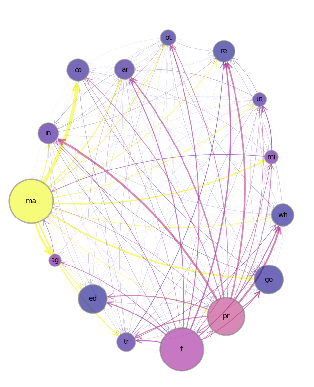
<Figure size 800x1000 with 1 Axes> — Figure 1:US 15 sector production network

Label	Sector	Label	Sector	Label	Sector
ag	Agriculture	wh	Wholesale	pr	Professional Services
mi	Mining	re	Retail	ed	Education & Health
ut	Utilities	tr	Transportation	ar	Arts & Entertainment
co	Construction	in	Information	ot	Other Services (exc govt)
ma	Manufacturing	fi	Finance	go	Government

An arrow from $i$ to $j$ means that some of sector $i$ ’s output serves as an input to production of sector $j$ .

Economies are characterised by many such links.

A basic framework for their analysis is Leontief’s input-output model.

After introducing the input-output model, we describe some of its connections to linear programming lecture.

39.2Input-output analysis¶

Let

$x_0$ be the amount of a single exogenous input to production, say labor
$x_j, j = 1,\ldots n$ be the gross output of final good $j$
$d_j, j = 1,\ldots n$ be the net output of final good $j$ that is available for final consumption
$z_{ij}$ be the quantity of good $i$ allocated to be an input to producing good $j$ for $i=1, \ldots n$ , $j = 1, \ldots n$
$z_{0j}$ be the quantity of labor allocated to producing good $j$ .
$a_{ij}$ be the number of units of good $i$ required to produce one unit of good $j$ , $i=0, \ldots, n, j= 1, \ldots n$ .
$w >0$ be an exogenous wage of labor, denominated in dollars per unit of labor
$p$ be an $n \times 1$ vector of prices of produced goods $i = 1, \ldots , n$ .

The technology for producing good $j \in \{1, \ldots , n\}$ is described by the Leontief function

x_j = \min_{i \in \{0, \ldots , n \}} \left( \frac{z_{ij}}{a_{ij}}\right)

(1)

39.2.1Two goods¶

To illustrate, we begin by setting $n =2$ and formulating the following network.

Source

G = nx.DiGraph()

nodes= (1, 2, 'c')
edges = ((1, 1), (1, 2), (2, 1), (2, 2), (1, 'c'), (2, 'c'))
edges1 = ((1, 1), (1, 2), (2, 1), (2, 2), (1, 'c'))
edges2 = [(2,'c')]
G.add_nodes_from(nodes)
G.add_edges_from(edges)

pos_list = ([0, 0], [2, 0], [1, -1])
pos = dict(zip(G.nodes(), pos_list))

fig, ax = plt.subplots()
plt.axis("off")

nx.draw_networkx_nodes(G, pos=pos, node_size=800,
                       node_color='white', edgecolors='black')
nx.draw_networkx_labels(G, pos=pos)
nx.draw_networkx_edges(G,pos=pos, edgelist=edges1,
                       node_size=300, connectionstyle='arc3,rad=0.2',
                       arrowsize=10, min_target_margin=15)
nx.draw_networkx_edges(G, pos=pos, edgelist=edges2,
                       node_size=300, connectionstyle='arc3,rad=-0.2',
                       arrowsize=10, min_target_margin=15)

plt.text(0.055, 0.125, r'$z_{11}$')
plt.text(1.825, 0.125, r'$z_{22}$')
plt.text(0.955, 0.1, r'$z_{21}$')
plt.text(0.955, -0.125, r'$z_{12}$')
plt.text(0.325, -0.5, r'$d_{1}$')
plt.text(1.6, -0.5, r'$d_{2}$')

plt.show()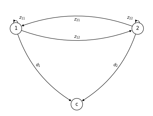

Feasible allocations must satisfy

\begin{aligned} (1 - a_{11}) x_1 - a_{12} x_2 & \geq d_1 \cr -a_{21} x_1 + (1 - a_{22}) x_2 & \geq d_2 \cr a_{01} x_1 + a_{02} x_2 & \leq x_0 \end{aligned}

(2)

This can be graphically represented as follows.

Source

fig, ax = plt.subplots()
ax.grid()

# Draw constraint lines
ax.hlines(0, -1, 400)
ax.vlines(0, -1, 200)

ax.plot(np.linspace(55, 380, 100), (50-0.9*np.linspace(55, 380, 100))/(-1.46), color="r")
ax.plot(np.linspace(-1, 400, 100), (60+0.16*np.linspace(-1, 400, 100))/0.83, color="r")
ax.plot(np.linspace(250, 395, 100), (62-0.04*np.linspace(250, 395, 100))/0.33, color="b")

ax.text(130, 38, r"$(1-a_{11})x_1 + a_{12}x_2 \geq d_1$", size=10)
ax.text(10, 105, r"$-a_{21}x_1 + (1-a_{22})x_2 \geq d_2$", size=10)
ax.text(150, 150, r"$a_{01}x_1 +a_{02}x_2 \leq x_0$", size=10)

# Draw the feasible region
feasible_set = Polygon(np.array([[301, 151],
                                 [368, 143],
                                 [250, 120]]),
                       color="cyan")
ax.add_patch(feasible_set)

# Draw the optimal solution
ax.plot(250, 120, "*", color="black")
ax.text(260, 115, "solution", size=10)

plt.show()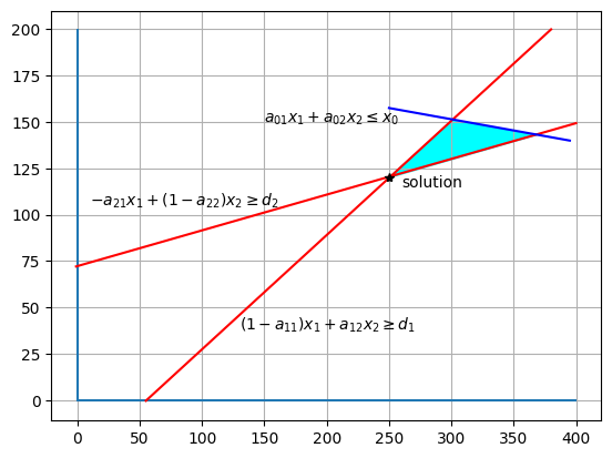

More generally, constraints on production are

\begin{aligned} (I - A) x & \geq d \cr a_0^\top x & \leq x_0 \end{aligned}

(3)

where $A$ is the $n \times n$ matrix with typical element $a_{ij}$ and $a_0^\top = \begin{bmatrix} a_{01} & \cdots & a_{0n} \end{bmatrix}$ .

If we solve the first block of equations of (3) for gross output $x$ we get

x = (I -A)^{-1} d \equiv L d

(4)

where the matrix $L = (I-A)^{-1}$ is sometimes called a Leontief Inverse.

To assure that the solution $X$ of (4) is a positive vector, the following Hawkins-Simon conditions suffice:

\begin{aligned} \det (I - A) > 0 \text{ and} \;\;\; \\ (I-A)_{ij} > 0 \text{ for all } i=j \end{aligned}

(5)

A = np.array([[0.1, 40],
             [0.01, 0]])
d = np.array([50, 2]).reshape((2, 1))

I = np.identity(2)
B = I - A
B

array([[ 9.e-01, -4.e+01],
       [-1.e-02,  1.e+00]])

Let’s check the Hawkins-Simon conditions

np.linalg.det(B) > 0 # checking Hawkins-Simon conditions

np.True_

Now, let’s compute the Leontief inverse matrix

L = np.linalg.inv(B) # obtaining Leontief inverse matrix
L

array([[2.0e+00, 8.0e+01],
       [2.0e-02, 1.8e+00]])

x = L @ d   # solving for gross output
x

array([[260. ],
       [  4.6]])

39.3Production possibility frontier¶

The second equation of (3) can be written

a_0^\top x = x_0

(7)

A_0^\top d = x_0

(8)

where

A_0^\top = a_0^\top (I - A)^{-1}

(9)

For $i \in \{1, \ldots , n\}$ , the $i$ th component of $A_0$ is the amount of labor that is required to produce one unit of final output of good $i$ .

Equation (8) sweeps out a production possibility frontier of final consumption bundles $d$ that can be produced with exogenous labor input $x_0$ .

Then we can find $A_0^\top$ by

a0 = np.array([4, 100])
A0 = a0 @ L
A0

array([ 10., 500.])

Thus, the production possibility frontier for this economy is

10d_1 + 500d_2 = x_0

(11)

39.4Prices¶

Dorfman et al. (1958) argue that relative prices of the $n$ produced goods must satisfy

\begin{aligned} p_1 = a_{11}p_1 + a_{21}p_2 + a_{01}w \\ p_2 = a_{12}p_1 + a_{22}p_2 + a_{02}w \end{aligned}

(12)

More generally,

p = A^\top p + a_0 w

(13)

which states that the price of each final good equals the total cost of production, which consists of costs of intermediate inputs $A^\top p$ plus costs of labor $a_0 w$ .

This equation can be written as

(I - A^\top) p = a_0 w

(14)

which implies

p = (I - A^\top)^{-1} a_0 w

(15)

Notice how (14) with (3) forms a conjugate pair through the appearance of operators that are transposes of one another.

This connection surfaces again in a classic linear program and its dual.

39.5Linear programs¶

A primal problem is

\min_{x} w a_0^\top x

(16)

subject to

(I - A) x \geq d

(17)

The associated dual problem is

\max_{p} p^\top d

(18)

subject to

(I -A)^\top p \leq a_0 w

(19)

The primal problem chooses a feasible production plan to minimize costs for delivering a pre-assigned vector of final goods consumption $d$ .

The dual problem chooses prices to maximize the value of a pre-assigned vector of final goods $d$ subject to prices covering costs of production.

By the strong duality theorem, optimal value of the primal and dual problems coincide:

w a_0^\top x^* = p^* d

(20)

where $^*$ 's denote optimal choices for the primal and dual problems.

The dual problem can be graphically represented as follows.

Source

fig, ax = plt.subplots()
ax.grid()

# Draw constraint lines
ax.hlines(0, -1, 50)
ax.vlines(0, -1, 250)

ax.plot(np.linspace(4.75, 49, 100), (4-0.9*np.linspace(4.75, 49, 100))/(-0.16), color="r")
ax.plot(np.linspace(0, 50, 100), (33+1.46*np.linspace(0, 50, 100))/0.83, color="r")

ax.text(15, 175, r"$(1-a_{11})p_1 - a_{21}p_2 \leq a_{01}w$", size=10)
ax.text(30, 85, r"$-a_{12}p_1 + (1-a_{22})p_2 \leq a_{02}w$", size=10)

# Draw the feasible region
feasible_set = Polygon(np.array([[17, 69],
                                 [4, 0],
                                 [0,0],
                                 [0, 40]]),
                       color="cyan")
ax.add_patch(feasible_set)

# Draw the optimal solution
ax.plot(17, 69, "*", color="black")
ax.text(18, 60, "dual solution", size=10)

plt.show()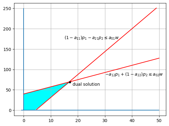

39.6Leontief inverse¶

We have discussed that gross output $x$ is given by (4), where $L$ is called the Leontief Inverse.

Recall the Neumann Series Lemma which states that $L$ exists if the spectral radius $r(A)<1$ .

In fact

L = \sum_{i=0}^{\infty} A^i

(21)

39.6.1Demand shocks¶

Consider the impact of a demand shock $\Delta d$ which shifts demand from $d_0$ to $d_1 = d_0 + \Delta d$ .

Gross output shifts from $x_0 = Ld_0$ to $x_1 = Ld_1$ .

If $r(A) < 1$ then a solution exists and

\Delta x = L \Delta d = \Delta d + A(\Delta d) + A^2 (\Delta d) + \cdots

(22)

This illustrates that an element $l_{ij}$ of $L$ shows the total impact on sector $i$ of a unit change in demand of good $j$ .

39.7Applications of graph theory¶

We can further study input-output networks through applications of graph theory.

An input-output network can be represented by a weighted directed graph induced by the adjacency matrix $A$ .

The set of nodes $V = [n]$ is the list of sectors and the set of edges is given by

E = \{(i,j) \in V \times V : a_{ij}>0\}

(23)

In Fig. 1 weights are indicated by the widths of the arrows, which are proportional to the corresponding input-output coefficients.

We can now use centrality measures to rank sectors and discuss their importance relative to the other sectors.

39.7.1Eigenvector centrality¶

Eigenvector centrality of a node $i$ is measured by

\begin{aligned} e_i = \frac{1}{r(A)} \sum_{1 \leq j \leq n} a_{ij} e_j \end{aligned}

(24)

We plot a bar graph of hub-based eigenvector centrality for the sectors represented in Fig. 1.

Source

fig, ax = plt.subplots()
ax.bar(codes, centrality, color=color_list, alpha=0.6)
ax.set_ylabel("eigenvector centrality", fontsize=12)
plt.show()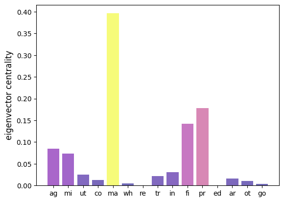

A higher measure indicates higher importance as a supplier.

As a result demand shocks in most sectors will significantly impact activity in sectors with high eigenvector centrality.

The above figure indicates that manufacturing is the most dominant sector in the US economy.

39.7.2Output multipliers¶

Another way to rank sectors in input-output networks is via output multipliers.

The output multiplier of sector $j$ denoted by $\mu_j$ is usually defined as the total sector-wide impact of a unit change of demand in sector $j$ .

Earlier when disussing demand shocks we concluded that for $L = (l_{ij})$ the element $l_{ij}$ represents the impact on sector $i$ of a unit change in demand in sector $j$ .

Thus,

\mu_j = \sum_{j=1}^n l_{ij}

(25)

This can be written as $\mu^\top = \mathbb{1}^\top L$ or

\mu^\top = \mathbb{1}^\top (I-A)^{-1}

(26)

Please note that here we use $\mathbb{1}$ to represent a vector of ones.

High ranking sectors within this measure are important buyers of intermediate goods.

A demand shock in such sectors will cause a large impact on the whole production network.

The following figure displays the output multipliers for the sectors represented in Fig. 1.

Source

A, F = build_coefficient_matrices(Z, X)
omult = qbn_io.katz_centrality(A, authority=True)

fig, ax = plt.subplots()
omult_color_list = qbn_io.colorise_weights(omult,beta=False)
ax.bar(codes, omult, color=omult_color_list, alpha=0.6)
ax.set_ylabel("Output multipliers", fontsize=12)
plt.show()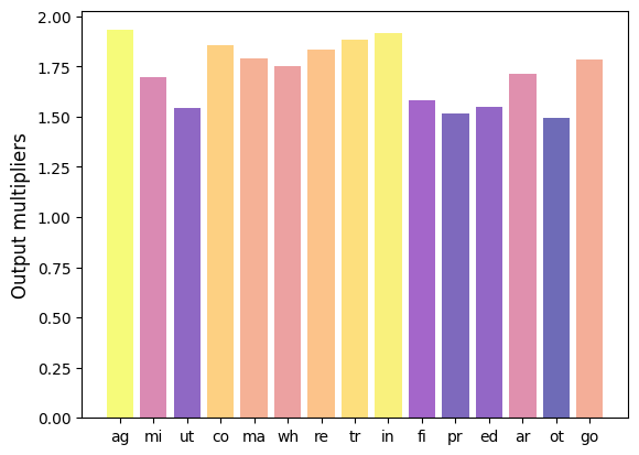

We observe that manufacturing and agriculture are highest ranking sectors.

39.8Exercises¶

Exercise 1

Dorfman et al. (1958) Chapter 9 discusses an example with the following parameter settings:

A = \begin{bmatrix} 0.1 & 1.46 \\ 0.16 & 0.17 \end{bmatrix} \text{ and } a_0 = \begin{bmatrix} .04 & .33 \end{bmatrix}

(27)

x = \begin{bmatrix} 250 \\ 120 \end{bmatrix} \text{ and } x_0 = 50

(28)

d = \begin{bmatrix} 50 \\ 60 \end{bmatrix}

(29)

Describe how they infer the input-output coefficients in $A$ and $a_0$ from the following hypothetical underlying “data” on agricultural and manufacturing industries:

z = \begin{bmatrix} 25 & 175 \\ 40 & 20 \end{bmatrix} \text{ and } z_0 = \begin{bmatrix} 10 & 40 \end{bmatrix}

(30)

where $z_0$ is a vector of labor services used in each industry.

Solution to Exercise 1

For each $i = 0,1,2$ and $j = 1,2$

a_{ij} = \frac{z_{ij}}{x_j}

(31)

Solution to Exercise 2

A = np.array([[0.1, 1.46],
              [0.16, 0.17]])
a_0 = np.array([0.04, 0.33])

I = np.identity(2)
B = I - A
L = np.linalg.inv(B)

A_0 = a_0 @ L
A_0

array([0.16751071, 0.69224776])

Thus the production possibility frontier is given by

0.17 d_1 + 0.69 d_2 = 50

(32)

References¶

Dorfman, R., Samuelson, P. A., & Solow, R. M. (1958). Linear Programming and Economic Analysis: Revised Edition. McGraw Hill.

CC-BY-SA-4.0 — Creative Commons License – This work is licensed under a Creative Commons Attribution-ShareAlike 4.0 International.

39. Input-Output Models

39.1Overview¶

39.2Input-output analysis¶

39.2.1Two goods¶

39.3Production possibility frontier¶

39.4Prices¶

39.5Linear programs¶

39.6Leontief inverse¶

39.6.1Demand shocks¶

39.7Applications of graph theory¶

39.7.1Eigenvector centrality¶

39.7.2Output multipliers¶

39.8Exercises¶