27. Commodity Prices
27.1Outline
For more than half of all countries around the globe, commodities account for the majority of total exports.
Examples of commodities include copper, diamonds, iron ore, lithium, cotton and coffee beans.
In this lecture we give an introduction to the theory of commodity prices.
The lecture is quite advanced relative to other lectures in this series.
We need to compute an equilibrium, and that equilibrium is described by a price function.
We will solve an equation where the price function is the unknown.
This is harder than solving an equation for an unknown number, or vector.
The lecture will discuss one way to solve a functional equation (an equation where the unknown object is a function).
For this lecture we need the yfinance library.
!pip install yfinanceOutput
Requirement already satisfied: yfinance in /opt/hostedtoolcache/Python/3.12.9/x64/lib/python3.12/site-packages (0.2.53)
Requirement already satisfied: pandas>=1.3.0 in /opt/hostedtoolcache/Python/3.12.9/x64/lib/python3.12/site-packages (from yfinance) (2.2.3)
Requirement already satisfied: numpy>=1.16.5 in /opt/hostedtoolcache/Python/3.12.9/x64/lib/python3.12/site-packages (from yfinance) (2.1.3)
Requirement already satisfied: requests>=2.31 in /opt/hostedtoolcache/Python/3.12.9/x64/lib/python3.12/site-packages (from yfinance) (2.32.3)
Requirement already satisfied: multitasking>=0.0.7 in /opt/hostedtoolcache/Python/3.12.9/x64/lib/python3.12/site-packages (from yfinance) (0.0.11)
Requirement already satisfied: platformdirs>=2.0.0 in /opt/hostedtoolcache/Python/3.12.9/x64/lib/python3.12/site-packages (from yfinance) (4.3.6)
Requirement already satisfied: pytz>=2022.5 in /opt/hostedtoolcache/Python/3.12.9/x64/lib/python3.12/site-packages (from yfinance) (2025.1)
Requirement already satisfied: frozendict>=2.3.4 in /opt/hostedtoolcache/Python/3.12.9/x64/lib/python3.12/site-packages (from yfinance) (2.4.6)
Requirement already satisfied: peewee>=3.16.2 in /opt/hostedtoolcache/Python/3.12.9/x64/lib/python3.12/site-packages (from yfinance) (3.17.9)
Requirement already satisfied: beautifulsoup4>=4.11.1 in /opt/hostedtoolcache/Python/3.12.9/x64/lib/python3.12/site-packages (from yfinance) (4.13.3)
Requirement already satisfied: soupsieve>1.2 in /opt/hostedtoolcache/Python/3.12.9/x64/lib/python3.12/site-packages (from beautifulsoup4>=4.11.1->yfinance) (2.6)
Requirement already satisfied: typing-extensions>=4.0.0 in /opt/hostedtoolcache/Python/3.12.9/x64/lib/python3.12/site-packages (from beautifulsoup4>=4.11.1->yfinance) (4.12.2)
Requirement already satisfied: python-dateutil>=2.8.2 in /opt/hostedtoolcache/Python/3.12.9/x64/lib/python3.12/site-packages (from pandas>=1.3.0->yfinance) (2.9.0.post0)
Requirement already satisfied: tzdata>=2022.7 in /opt/hostedtoolcache/Python/3.12.9/x64/lib/python3.12/site-packages (from pandas>=1.3.0->yfinance) (2025.1)
Requirement already satisfied: charset-normalizer<4,>=2 in /opt/hostedtoolcache/Python/3.12.9/x64/lib/python3.12/site-packages (from requests>=2.31->yfinance) (3.4.1)
Requirement already satisfied: idna<4,>=2.5 in /opt/hostedtoolcache/Python/3.12.9/x64/lib/python3.12/site-packages (from requests>=2.31->yfinance) (3.10)
Requirement already satisfied: urllib3<3,>=1.21.1 in /opt/hostedtoolcache/Python/3.12.9/x64/lib/python3.12/site-packages (from requests>=2.31->yfinance) (2.3.0)
Requirement already satisfied: certifi>=2017.4.17 in /opt/hostedtoolcache/Python/3.12.9/x64/lib/python3.12/site-packages (from requests>=2.31->yfinance) (2025.1.31)
Requirement already satisfied: six>=1.5 in /opt/hostedtoolcache/Python/3.12.9/x64/lib/python3.12/site-packages (from python-dateutil>=2.8.2->pandas>=1.3.0->yfinance) (1.17.0)
We will use the following imports
import numpy as np
import yfinance as yf
import matplotlib.pyplot as plt
from scipy.interpolate import interp1d
from scipy.optimize import brentq
from scipy.stats import beta27.2Data
The figure below shows the price of cotton in USD since the start of 2016.
Source
s = yf.download('CT=F', '2016-1-1', '2023-4-1')['Close']Output
YF.download() has changed argument auto_adjust default to True
Source
fig, ax = plt.subplots()

ax.plot(s, marker='o', alpha=0.5, ms=1)
ax.set_ylabel('cotton price in USD', fontsize=12)
ax.set_xlabel('date', fontsize=12)

plt.show()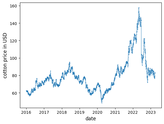
The figure shows surprisingly large movements in the price of cotton.
What causes these movements?
In general, prices depend on the choices and actions of
- suppliers,
- consumers, and
- speculators.
Our focus will be on the interaction between these parties.
We will connect them together in a dynamic model of supply and demand, called the competitive storage model.
This model was developed by Samuelson (1971), Wright & Williams (1982), Scheinkman & Schechtman (1983), Deaton & Laroque (1992), Deaton & Laroque (1996), and Chambers & Bailey (1996).
27.3The competitive storage model
In the competitive storage model, commodities are assets that
- can be traded by speculators and
- have intrinsic value to consumers.
Total demand is the sum of consumer demand and demand by speculators.
Supply is exogenous, depending on “harvests”.
The equilibrium price is determined competitively.
It is a function of the current state (which determines current harvests and predicts future harvests).
27.4The model
Consider a market for a single commodity, whose price is given at by .
The harvest of the commodity at time is .
We assume that the sequence is IID with common density function ϕ, where ϕ is nonnegative.
Speculators can store the commodity between periods, with units purchased in the current period yielding units in the next.
Here the parameter is a depreciation rate for the commodity.
For simplicity, the risk free interest rate is taken to be zero, so expected profit on purchasing units is
Here is the expectation of taken at time .
27.5Equilibrium
In this section we define the equilibrium and discuss how to compute it.
27.5.1Equilibrium conditions
Speculators are assumed to be risk neutral, which means that they buy the commodity whenever expected profits are positive.
As a consequence, if expected profits are positive, then the market is not in equilibrium.
Hence, to be in equilibrium, prices must satisfy the “no-arbitrage” condition
This means that if the expected price is lower than the current price, there is no room for arbitrage.
Profit maximization gives the additional condition
We also require that the market clears, with supply equaling demand in each period.
We assume that consumers generate demand quantity corresponding to price .
Let be the inverse demand function.
Regarding quantities,
- supply is the sum of carryover by speculators and the current harvest, and
- demand is the sum of purchases by consumers and purchases by speculators.
Mathematically,
- supply is given by , which takes values in , while
- demand
Thus, the market equilibrium condition is
The initial condition is treated as given.
27.5.2An equilibrium function
How can we find an equilibrium?
Our path of attack will be to seek a system of prices that depend only on the current state.
(Our solution method involves using an ansatz, which is an educated guess --- in this case for the price function.)
In other words, we take a function on and set for every .
Prices and quantities then follow
We choose so that these prices and quantities satisfy the equilibrium conditions above.
More precisely, we seek a such that (2) and (3) hold for the corresponding system (5).
where
It turns out that such a will suffice, in the sense that (2) and (3) hold for the corresponding system (5).
To see this, observe first that
Thus (2) requires that
This inequality is immediate from (6).
Second, regarding (3), suppose that
Then by (6) we have
But then and .
As a consequence, both (2) and (3) hold.
We have found an equilibrium, which verifies the ansatz.
27.5.3Computing the equilibrium
We now know that an equilibrium can be obtained by finding a function that satisfies (6).
It can be shown that, under mild conditions there is exactly one function on satisfying (6).
Moreover, we can compute this function using successive approximation.
This means that we start with a guess of the function and then update it using (6).
This generates a sequence of functions
We continue until this process converges, in the sense that and are very close together.
Then we take the final that we computed as our approximation of .
To implement our update step, it is helpful if we put (6) and (7) together.
This leads us to the update rule
In other words, we take as given and, at each , solve for in
Actually we can’t do this at every , so instead we do it on a grid of points .
Then we get the corresponding values .
Then we compute as the linear interpolation of the values over the grid .
Then we repeat, seeking convergence.
27.6Code
The code below implements this iterative process, starting from .
The distribution ϕ is set to a shifted Beta distribution (although many other choices are possible).
The integral in (12) is computed via Monte Carlo.
α, a, c = 0.8, 1.0, 2.0
beta_a, beta_b = 5, 5
mc_draw_size = 250
gridsize = 150
grid_max = 35
grid = np.linspace(a, grid_max, gridsize)

beta_dist = beta(5, 5)
Z = a + beta_dist.rvs(mc_draw_size) * c    # Shock observations
D = P = lambda x: 1.0 / x
tol = 1e-4


def T(p_array):

    new_p = np.empty_like(p_array)

    # Interpolate to obtain p as a function.
    p = interp1d(grid,
                 p_array,
                 fill_value=(p_array[0], p_array[-1]),
                 bounds_error=False)

    # Update
    for i, x in enumerate(grid):

        h = lambda q: q - max(α * np.mean(p(α * (x - D(q)) + Z)), P(x))
        new_p[i] = brentq(h, 1e-8, 100)

    return new_p


fig, ax = plt.subplots()

price = P(grid)
ax.plot(grid, price, alpha=0.5, lw=1, label="inverse demand curve")
error = tol + 1
while error > tol:
    new_price = T(price)
    error = max(np.abs(new_price - price))
    price = new_price

ax.plot(grid, price, 'k-', alpha=0.5, lw=2, label=r'$p^*$')
ax.legend()
ax.set_xlabel('$x$')
ax.set_ylabel("prices")

plt.show()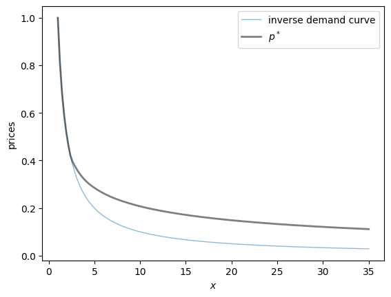
The figure above shows the inverse demand curve , which is also , as well as our approximation of .
Once we have an approximation of , we can simulate a time series of prices.
# Turn the price array into a price function
p_star = interp1d(grid,
                  price,
                  fill_value=(price[0], price[-1]),
                  bounds_error=False)

def carry_over(x):
    return α * (x - D(p_star(x)))

def generate_cp_ts(init=1, n=50):
    X = np.empty(n)
    X[0] = init
    for t in range(n-1):
            Z = a + c * beta_dist.rvs()
            X[t+1] = carry_over(X[t]) + Z
    return p_star(X)

fig, ax = plt.subplots()
ax.plot(generate_cp_ts(), label="price")
ax.set_xlabel("time")
ax.legend()
plt.show()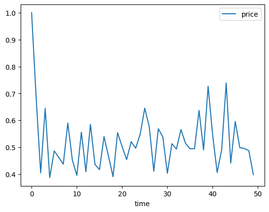
- Samuelson, P. A. (1971). Stochastic speculative price. Proceedings of the National Academy of Sciences, 68(2), 335–337.
- Wright, B. D., & Williams, J. C. (1982). The economic role of commodity storage. The Economic Journal, 92(367), 596–614.
- Scheinkman, J. A., & Schechtman, J. (1983). A simple competitive model with production and storage. The Review of Economic Studies, 50(3), 427–441.
- Deaton, A., & Laroque, G. (1992). On the behavior of commodity prices. The Review of Economic Studies, 59, 1–23.
- Deaton, A., & Laroque, G. (1996). Competitive storage and commodity price dynamics. Journal of Political Economy, 104(5), 896–923.
- Chambers, M. J., & Bailey, R. E. (1996). A theory of commodity price fluctuations. Journal of Political Economy, 104(5), 924–957.

Creative Commons License – This work is licensed under a Creative Commons Attribution-ShareAlike 4.0 International.