15. Monetarist Theory of Price Levels with Adaptive Expectations
15.1Overview
This lecture is a sequel or prequel to A Monetarist Theory of Price Levels.
We’ll use linear algebra to do some experiments with an alternative “monetarist” or “fiscal” theory of price levels.
Like the model in A Monetarist Theory of Price Levels, the model asserts that when a government persistently spends more than it collects in taxes and prints money to finance the shortfall, it puts upward pressure on the price level and generates persistent inflation.
Instead of the “perfect foresight” or “rational expectations” version of the model in A Monetarist Theory of Price Levels, our model in the present lecture is an “adaptive expectations” version of a model that Cagan (1956) used to study the monetary dynamics of hyperinflations.
It combines these components:
a demand function for real money balances that asserts that the logarithm of the quantity of real balances demanded depends inversely on the public’s expected rate of inflation
an adaptive expectations model that describes how the public’s anticipated rate of inflation responds to past values of actual inflation
an equilibrium condition that equates the demand for money to the supply
an exogenous sequence of rates of growth of the money supply
Our model stays quite close to Cagan’s original specification.
As in Present Values and Consumption Smoothing, the only linear algebra operations that we’ll be using are matrix multiplication and matrix inversion.
To facilitate using linear matrix algebra as our principal mathematical tool, we’ll use a finite horizon version of the model.
15.2Structure of the model
Let
- be the log of the supply of nominal money balances;
- be the net rate of growth of nominal balances;
- be the log of the price level;
- be the net rate of inflation between and ;
- be the public’s expected rate of inflation between and ;
- the horizon -- i.e., the last period for which the model will determine
- public’s initial expected rate of inflation between time 0 and time 1.
The demand for real balances is governed by the following version of the Cagan demand function
This equation asserts that the demand for real balances is inversely related to the public’s expected rate of inflation with sensitivity α.
Equating the logarithm of the demand for money to the logarithm of the supply of money in equation (1) and solving for the logarithm of the price level gives
Taking the difference between equation (2) at time and at time gives
We assume that the expected rate of inflation is governed by the following adaptive expectations scheme proposed by Friedman (1956) and Cagan (1956), where denotes the weight on expected inflation.
As exogenous inputs into the model, we take initial conditions and a money growth sequence .
As endogenous outputs of our model we want to find sequences as functions of the exogenous inputs.
We’ll do some mental experiments by studying how the model outputs vary as we vary the model inputs.
15.3Representing key equations with linear algebra
We begin by writing the equation (4) adaptive expectations model for for as
Write this equation as
where the matrix , the matrix , and the vectors are defined implicitly by aligning these two equations.
Next we write the key equation (3) in matrix notation as
Represent the previous equation system in terms of vectors and matrices as
where the matrix is defined implicitly to align this equation with the preceding equation system.
15.4Harvesting insights from our matrix formulation
We now have all of the ingredients we need to solve for π as a function of .
Combine equations (6)and (8) to get
which implies that
Multiplying both sides of the above equation by the inverse of the matrix on the left side gives
Having solved equation (11) for , we can use equation (8) to solve for π:
We have thus solved for two of the key endogenous time series determined by our model, namely, the sequence of expected inflation rates and the sequence π of actual inflation rates.
Knowing these, we can then quickly calculate the associated sequence of the logarithm of the price level from equation (2).
Let’s fill in the details for this step.
Since we now know μ it is easy to compute .
Thus, notice that we can represent the equations
as the matrix equation
Multiplying both sides of equation (14) with the inverse of the matrix on the left will give
Equation (15) shows that the log of the money supply at equals the log of the initial money supply plus accumulation of rates of money growth between times 0 and .
We can then compute for each from equation (2).
We can write a compact formula for as
where
which is just with the last element dropped.
15.5Forecast errors and model computation
Our computations will verify that
so that in general
This outcome is typical in models in which adaptive expectations hypothesis like equation (4) appear as a component.
In A Monetarist Theory of Price Levels, we studied a version of the model that replaces hypothesis (4) with a “perfect foresight” or “rational expectations” hypothesis.
But now, let’s dive in and do some computations with the adaptive expectations version of the model.
As usual, we’ll start by importing some Python modules.
import numpy as np
from collections import namedtuple
import matplotlib.pyplot as plt
Cagan_Adaptive = namedtuple("Cagan_Adaptive",
["α", "m0", "Eπ0", "T", "λ"])
def create_cagan_adaptive_model(α = 5, m0 = 1, Eπ0 = 0.5, T=80, λ = 0.9):
return Cagan_Adaptive(α, m0, Eπ0, T, λ)
md = create_cagan_adaptive_model()We solve the model and plot variables of interests using the following functions.
def solve_cagan_adaptive(model, μ_seq):
    " Solve the Cagan model in finite time. "
    α, m0, Eπ0, T, λ = model

    A = np.eye(T+2, T+2) - λ*np.eye(T+2, T+2, k=-1)
    B = np.eye(T+2, T+1, k=-1)
    C = -α*np.eye(T+1, T+2) + α*np.eye(T+1, T+2, k=1)
    Eπ0_seq = np.append(Eπ0, np.zeros(T+1))

    # Eπ_seq is of length T+2
    Eπ_seq = np.linalg.solve(A - (1-λ)*B @ C, (1-λ) * B @ μ_seq + Eπ0_seq)

    # π_seq is of length T+1
    π_seq = μ_seq + C @ Eπ_seq

    D = np.eye(T+1, T+1) - np.eye(T+1, T+1, k=-1) # D is the coefficient matrix in Equation (14.8)
    m0_seq = np.append(m0, np.zeros(T))

    # m_seq is of length T+2
    m_seq = np.linalg.solve(D, μ_seq + m0_seq)
    m_seq = np.append(m0, m_seq)

    # p_seq is of length T+2
    p_seq = m_seq + α * Eπ_seq

    return π_seq, Eπ_seq, m_seq, p_seq
def solve_and_plot(model, μ_seq):
π_seq, Eπ_seq, m_seq, p_seq = solve_cagan_adaptive(model, μ_seq)
T_seq = range(model.T+2)
fig, ax = plt.subplots(5, 1, figsize=[5, 12], dpi=200)
ax[0].plot(T_seq[:-1], μ_seq)
ax[1].plot(T_seq[:-1], π_seq, label=r'$\pi_t$')
ax[1].plot(T_seq, Eπ_seq, label=r'$\pi^{*}_{t}$')
ax[2].plot(T_seq, m_seq - p_seq)
ax[3].plot(T_seq, m_seq)
ax[4].plot(T_seq, p_seq)
y_labs = [r'$\mu$', r'$\pi$', r'$m - p$', r'$m$', r'$p$']
subplot_title = [r'Money supply growth', r'Inflation', r'Real balances', r'Money supply', r'Price level']
for i in range(5):
ax[i].set_xlabel(r'$t$')
ax[i].set_ylabel(y_labs[i])
ax[i].set_title(subplot_title[i])
ax[1].legend()
plt.tight_layout()
plt.show()
return π_seq, Eπ_seq, m_seq, p_seq15.6Technical condition for stability
In constructing our examples, we shall assume that satisfy
The source of this condition is the following string of deductions:
By assuring that the coefficient on is less than one in absolute value, condition (20) assures stability of the dynamics of described by the last line of our string of deductions.
The reader is free to study outcomes in examples that violate condition (20).
print(np.abs((md.λ - md.α*(1-md.λ))/(1 - md.α*(1-md.λ))))0.8
15.7Experiments
Now we’ll turn to some experiments.
15.7.1Experiment 1
We’ll study a situation in which the rate of growth of the money supply is from to and then permanently falls to at .
Thus, let .
So where , we assume that
Notice that we studied exactly this experiment in a rational expectations version of the model in A Monetarist Theory of Price Levels.
So by comparing outcomes across the two lectures, we can learn about consequences of assuming adaptive expectations, as we do here, instead of rational expectations as we assumed in that other lecture.
# Parameters for the experiment 1
T1 = 60
μ0 = 0.5
μ_star = 0

μ_seq_1 = np.append(μ0*np.ones(T1), μ_star*np.ones(md.T+1-T1))

# solve and plot
π_seq_1, Eπ_seq_1, m_seq_1, p_seq_1 = solve_and_plot(md, μ_seq_1)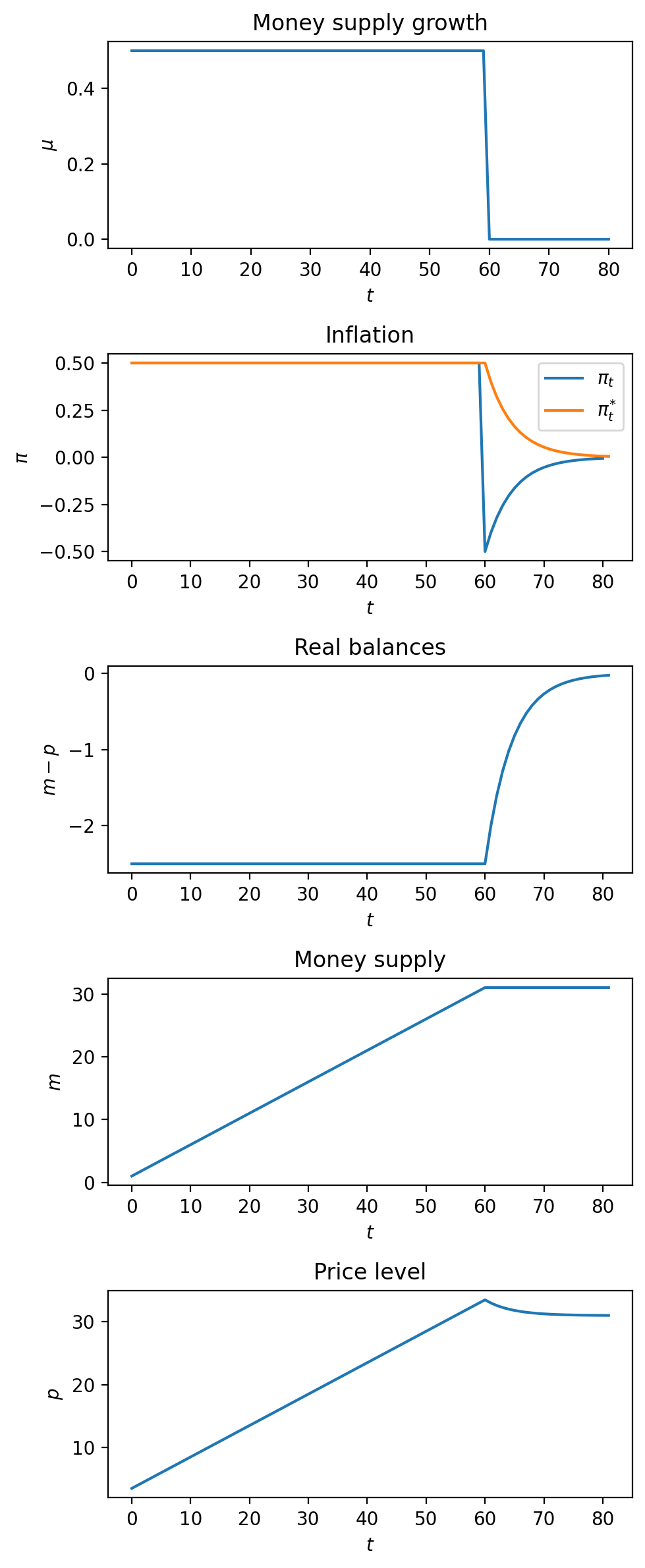
We invite the reader to compare outcomes with those under rational expectations studied in A Monetarist Theory of Price Levels.
Please note how the actual inflation rate “overshoots” its ultimate steady-state value at the time of the sudden reduction in the rate of growth of the money supply at time .
We invite you to explain to yourself the source of this overshooting and why it does not occur in the rational expectations version of the model.
15.7.2Experiment 2
Now we’ll do a different experiment, namely, a gradual stabilization in which the rate of growth of the money supply smoothly decline from a high value to a persistently low value.
While price level inflation eventually falls, it falls more slowly than the driving force that ultimately causes it to fall, namely, the falling rate of growth of the money supply.
The sluggish fall in inflation is explained by how anticipated inflation persistently exceeds actual inflation during the transition from a high inflation to a low inflation situation.
# parameters
ϕ = 0.9
μ_seq_2 = np.array([ϕ**t * μ0 + (1-ϕ**t)*μ_star for t in range(md.T)])
μ_seq_2 = np.append(μ_seq_2, μ_star)


# solve and plot
π_seq_2, Eπ_seq_2, m_seq_2, p_seq_2 = solve_and_plot(md, μ_seq_2)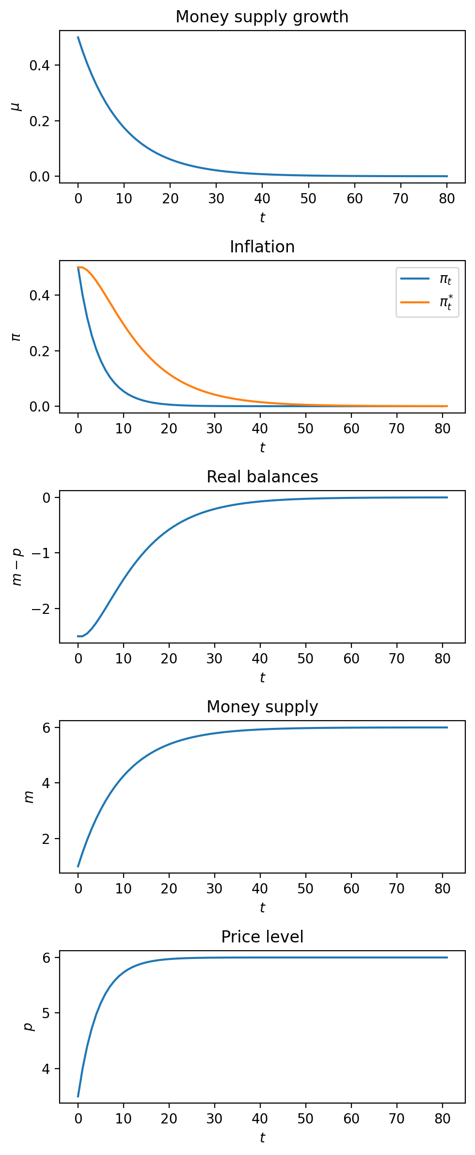
- Cagan, P. (1956). The Monetary Dynamics of Hyperinflation. In M. Friedman (Ed.), Studies in the Quantity Theory of Money (pp. 25–117). University of Chicago Press.
- Friedman, M. (1956). A Theory of the Consumption Function. Princeton University Press.

Creative Commons License – This work is licensed under a Creative Commons Attribution-ShareAlike 4.0 International.