41. Networks
!pip install quantecon-book-networks pandas-datareaderOutput
Collecting quantecon-book-networks
Using cached quantecon_book_networks-1.1-py2.py3-none-any.whl.metadata (1.3 kB)
Collecting pandas-datareader
  Using cached pandas_datareader-0.10.0-py3-none-any.whl.metadata (2.9 kB)
Requirement already satisfied: numpy in /opt/hostedtoolcache/Python/3.12.9/x64/lib/python3.12/site-packages (from quantecon-book-networks) (2.1.3)
Requirement already satisfied: scipy in /opt/hostedtoolcache/Python/3.12.9/x64/lib/python3.12/site-packages (from quantecon-book-networks) (1.15.2)
Requirement already satisfied: pandas in /opt/hostedtoolcache/Python/3.12.9/x64/lib/python3.12/site-packages (from quantecon-book-networks) (2.2.3)
Requirement already satisfied: matplotlib in /opt/hostedtoolcache/Python/3.12.9/x64/lib/python3.12/site-packages (from quantecon-book-networks) (3.10.0)
Requirement already satisfied: networkx in /opt/hostedtoolcache/Python/3.12.9/x64/lib/python3.12/site-packages (from quantecon-book-networks) (3.4.2)
Requirement already satisfied: quantecon in /opt/hostedtoolcache/Python/3.12.9/x64/lib/python3.12/site-packages (from quantecon-book-networks) (0.8.0)
Collecting POT (from quantecon-book-networks)
  Using cached POT-0.9.5-cp312-cp312-manylinux_2_17_x86_64.manylinux2014_x86_64.whl.metadata (34 kB)
Collecting lxml (from pandas-datareader)
Using cached lxml-5.3.1-cp312-cp312-manylinux_2_28_x86_64.whl.metadata (3.7 kB)
Requirement already satisfied: requests>=2.19.0 in /opt/hostedtoolcache/Python/3.12.9/x64/lib/python3.12/site-packages (from pandas-datareader) (2.32.3)
Requirement already satisfied: python-dateutil>=2.8.2 in /opt/hostedtoolcache/Python/3.12.9/x64/lib/python3.12/site-packages (from pandas->quantecon-book-networks) (2.9.0.post0)
Requirement already satisfied: pytz>=2020.1 in /opt/hostedtoolcache/Python/3.12.9/x64/lib/python3.12/site-packages (from pandas->quantecon-book-networks) (2025.1)
Requirement already satisfied: tzdata>=2022.7 in /opt/hostedtoolcache/Python/3.12.9/x64/lib/python3.12/site-packages (from pandas->quantecon-book-networks) (2025.1)
Requirement already satisfied: charset-normalizer<4,>=2 in /opt/hostedtoolcache/Python/3.12.9/x64/lib/python3.12/site-packages (from requests>=2.19.0->pandas-datareader) (3.4.1)
Requirement already satisfied: idna<4,>=2.5 in /opt/hostedtoolcache/Python/3.12.9/x64/lib/python3.12/site-packages (from requests>=2.19.0->pandas-datareader) (3.10)
Requirement already satisfied: urllib3<3,>=1.21.1 in /opt/hostedtoolcache/Python/3.12.9/x64/lib/python3.12/site-packages (from requests>=2.19.0->pandas-datareader) (2.3.0)
Requirement already satisfied: certifi>=2017.4.17 in /opt/hostedtoolcache/Python/3.12.9/x64/lib/python3.12/site-packages (from requests>=2.19.0->pandas-datareader) (2025.1.31)
Requirement already satisfied: contourpy>=1.0.1 in /opt/hostedtoolcache/Python/3.12.9/x64/lib/python3.12/site-packages (from matplotlib->quantecon-book-networks) (1.3.1)
Requirement already satisfied: cycler>=0.10 in /opt/hostedtoolcache/Python/3.12.9/x64/lib/python3.12/site-packages (from matplotlib->quantecon-book-networks) (0.12.1)
Requirement already satisfied: fonttools>=4.22.0 in /opt/hostedtoolcache/Python/3.12.9/x64/lib/python3.12/site-packages (from matplotlib->quantecon-book-networks) (4.56.0)
Requirement already satisfied: kiwisolver>=1.3.1 in /opt/hostedtoolcache/Python/3.12.9/x64/lib/python3.12/site-packages (from matplotlib->quantecon-book-networks) (1.4.8)
Requirement already satisfied: packaging>=20.0 in /opt/hostedtoolcache/Python/3.12.9/x64/lib/python3.12/site-packages (from matplotlib->quantecon-book-networks) (24.2)
Requirement already satisfied: pillow>=8 in /opt/hostedtoolcache/Python/3.12.9/x64/lib/python3.12/site-packages (from matplotlib->quantecon-book-networks) (11.1.0)
Requirement already satisfied: pyparsing>=2.3.1 in /opt/hostedtoolcache/Python/3.12.9/x64/lib/python3.12/site-packages (from matplotlib->quantecon-book-networks) (3.2.1)
Requirement already satisfied: numba>=0.49.0 in /opt/hostedtoolcache/Python/3.12.9/x64/lib/python3.12/site-packages (from quantecon->quantecon-book-networks) (0.61.0)
Requirement already satisfied: sympy in /opt/hostedtoolcache/Python/3.12.9/x64/lib/python3.12/site-packages (from quantecon->quantecon-book-networks) (1.13.3)
Requirement already satisfied: llvmlite<0.45,>=0.44.0dev0 in /opt/hostedtoolcache/Python/3.12.9/x64/lib/python3.12/site-packages (from numba>=0.49.0->quantecon->quantecon-book-networks) (0.44.0)
Requirement already satisfied: six>=1.5 in /opt/hostedtoolcache/Python/3.12.9/x64/lib/python3.12/site-packages (from python-dateutil>=2.8.2->pandas->quantecon-book-networks) (1.17.0)
Requirement already satisfied: mpmath<1.4,>=1.1.0 in /opt/hostedtoolcache/Python/3.12.9/x64/lib/python3.12/site-packages (from sympy->quantecon->quantecon-book-networks) (1.3.0)
Using cached quantecon_book_networks-1.1-py2.py3-none-any.whl (364 kB)
Using cached pandas_datareader-0.10.0-py3-none-any.whl (109 kB)
Using cached lxml-5.3.1-cp312-cp312-manylinux_2_28_x86_64.whl (5.0 MB)
Using cached POT-0.9.5-cp312-cp312-manylinux_2_17_x86_64.manylinux2014_x86_64.whl (901 kB)
Installing collected packages: lxml, POT, pandas-datareader, quantecon-book-networks
Successfully installed POT-0.9.5 lxml-5.3.1 pandas-datareader-0.10.0 quantecon-book-networks-1.1
41.1Outline
In recent years there has been rapid growth in a field called network science.
Network science studies relationships between groups of objects.
One important example is the world wide web , where web pages are connected by hyperlinks.
Another is the human brain: studies of brain function emphasize the network of connections between nerve cells (neurons).
Artificial neural networks are based on this idea, using data to build intricate connections between simple processing units.
Epidemiologists studying transmission of diseases like COVID-19 analyze interactions between groups of human hosts.
In operations research, network analysis is used to study fundamental problems as on minimum cost flow, the traveling salesman, shortest paths, and assignment.
This lecture gives an introduction to economic and financial networks.
Some parts of this lecture are drawn from the text
https://
We will need the following imports.
import numpy as np
import networkx as nx
import matplotlib.pyplot as plt
import pandas as pd
import quantecon as qe

import matplotlib.cm as cm
import quantecon_book_networks.input_output as qbn_io
import quantecon_book_networks.data as qbn_data

import matplotlib.patches as mpatches41.2Economic and financial networks
Within economics, important examples of networks include
- financial networks
- production networks
- trade networks
- transport networks and
- social networks
Social networks affect trends in market sentiment and consumer decisions.
The structure of financial networks helps to determine relative fragility of the financial system.
The structure of production networks affects trade, innovation and the propagation of local shocks.
To better understand such networks, let’s look at some examples in more depth.
41.2.1Example: Aircraft Exports
The following figure shows international trade in large commercial aircraft in 2019 based on International Trade Data SITC Revision 2.
Source
ch1_data = qbn_data.introduction()
export_figures = False

DG = ch1_data['aircraft_network']
pos = ch1_data['aircraft_network_pos']

centrality = nx.eigenvector_centrality(DG)
node_total_exports = qbn_io.node_total_exports(DG)
edge_weights = qbn_io.edge_weights(DG)

node_pos_dict = pos

node_sizes = qbn_io.normalise_weights(node_total_exports,10000)
edge_widths = qbn_io.normalise_weights(edge_weights,10)

node_colors = qbn_io.colorise_weights(list(centrality.values()),color_palette=cm.viridis)
node_to_color = dict(zip(DG.nodes,node_colors))
edge_colors = []
for src,_ in DG.edges:
    edge_colors.append(node_to_color[src])

fig, ax = plt.subplots(figsize=(10, 10))
ax.axis('off')

nx.draw_networkx_nodes(DG,
                       node_pos_dict,
                       node_color=node_colors,
                       node_size=node_sizes,
                       linewidths=2,
                       alpha=0.6,
                       ax=ax)

nx.draw_networkx_labels(DG,
                        node_pos_dict,
                        ax=ax)

nx.draw_networkx_edges(DG,
                       node_pos_dict,
                       edge_color=edge_colors,
                       width=edge_widths,
                       arrows=True,
                       arrowsize=20,
                       ax=ax,
                       arrowstyle='->',
                       node_size=node_sizes,
                       connectionstyle='arc3,rad=0.15')

plt.show()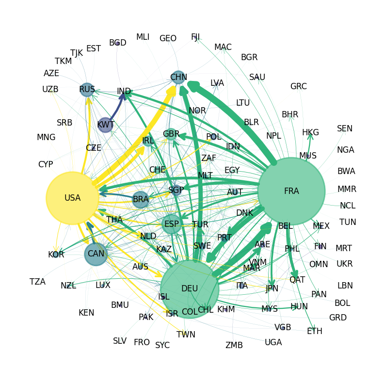
Figure 1:Commercial Aircraft Network
The circles in the figure are called nodes or vertices -- in this case they represent countries.
The arrows in the figure are called edges or links.
Node size is proportional to total exports and edge width is proportional to exports to the target country.
(The data is for trade in commercial aircraft weighing at least 15,000kg and was sourced from CID Dataverse.)
The figure shows that the US, France and Germany are major export hubs.
In the discussion below, we learn to quantify such ideas.
41.2.2Example: A Markov Chain
Recall that, in our lecture on Markov chains we studied a dynamic model of business cycles where the states are
- “ng” = “normal growth”
- “mr” = “mild recession”
- “sr” = “severe recession”
Let’s examine the following figure
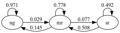
This is an example of a network, where the set of nodes equals the states:
The edges between the nodes show the one month transition probabilities.
41.3An introduction to graph theory
Now we’ve looked at some examples, let’s move on to theory.
This theory will allow us to better organize our thoughts.
The theoretical part of network science is constructed using a major branch of mathematics called graph theory.
Graph theory can be complicated and we will cover only the basics.
However, these concepts will already be enough for us to discuss interesting and important ideas on economic and financial networks.
We focus on “directed” graphs, where connections are, in general, asymmetric (arrows typically point one way, not both ways).
E.g.,
- bank lends money to bank
- firm supplies goods to firm
- individual “follows” individual on a given social network
(“Undirected” graphs, where connections are symmetric, are a special case of directed graphs --- we just need to insist that each arrow pointing from to is paired with another arrow pointing from to .)
41.3.1Key definitions
A directed graph consists of two things:
- a finite set and
- a collection of pairs where and are elements of .
The elements of are called the vertices or nodes of the graph.
The pairs are called the edges of the graph and the set of all edges will usually be denoted by
Intuitively and visually, an edge is understood as an arrow from node to node .
(A neat way to represent an arrow is to record the location of the tail and head of the arrow, and that’s exactly what an edge does.)
In the aircraft export example shown in Fig. 1
- is all countries included in the data set.
- is all the arrows in the figure, each indicating some positive amount of aircraft exports from one country to another.
Let’s look at more examples.
Two graphs are shown below, each with three nodes.
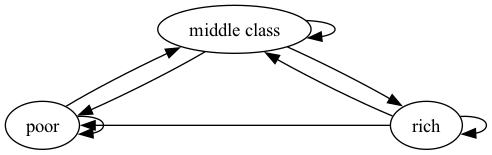
Figure 2:Poverty Trap
We now construct a graph with the same nodes but different edges.
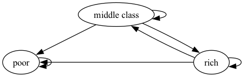
Figure 3:Poverty Trap
For these graphs, the arrows (edges) can be thought of as representing positive transition probabilities over a given unit of time.
In general, if an edge exists, then the node is called a direct predecessor of and is called a direct successor of .
Also, for ,
- the in-degree is the number of direct predecessors of and
- the out-degree is the number of direct successors of .
41.3.2Digraphs in Networkx
The Python package Networkx provides a convenient data structure for representing directed graphs and implements many common routines for analyzing them.
As an example, let us recreate Fig. 3 using Networkx.
To do so, we first create an empty DiGraph object:
G_p = nx.DiGraph()Next we populate it with nodes and edges.
To do this we write down a list of all edges, with poor represented by p and so on:
edge_list = [('p', 'p'),
             ('m', 'p'), ('m', 'm'), ('m', 'r'),
             ('r', 'p'), ('r', 'm'), ('r', 'r')]
Finally, we add the edges to our DiGraph object:
for e in edge_list:
    u, v = e
    G_p.add_edge(u, v)
Alternatively, we can use the method add_edges_from.
G_p.add_edges_from(edge_list)Adding the edges automatically adds the nodes, so G_p is now a
correct representation of our graph.
We can verify this by plotting the graph via Networkx with the following code:
fig, ax = plt.subplots()
nx.draw_spring(G_p, ax=ax, node_size=500, with_labels=True,
               font_weight='bold', arrows=True, alpha=0.8,
               connectionstyle='arc3,rad=0.25', arrowsize=20)
plt.show()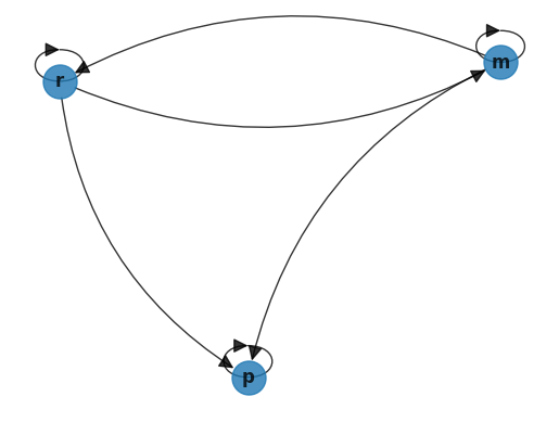
The figure obtained above matches the original directed graph in Fig. 3.
DiGraph objects have methods that calculate in-degree and out-degree
of nodes.
For example,
G_p.in_degree('p')341.3.3Communication
Next, we study communication and connectedness, which have important implications for economic networks.
Node is called accessible from node if either or there exists a sequence of edges that lead from to .
- in this case, we write
(Visually, there is a sequence of arrows leading from to .)
For example, suppose we have a directed graph representing a production network, where
- elements of are industrial sectors and
- existence of an edge means that supplies products or services to .
Then means that sector is an upstream supplier of sector .
Two nodes and are said to communicate if both and .
A graph is called strongly connected if all nodes communicate.
For example, Fig. 2 is strongly connected however in Fig. 3 rich is not accessible from poor, thus it is not strongly connected.
We can verify this by first constructing the graphs using Networkx and then using nx.is_strongly_connected.
fig, ax = plt.subplots()
G1 = nx.DiGraph()

G1.add_edges_from([('p', 'p'),('p','m'),('p','r'),
             ('m', 'p'), ('m', 'm'), ('m', 'r'),
             ('r', 'p'), ('r', 'm'), ('r', 'r')])

nx.draw_networkx(G1, with_labels = True)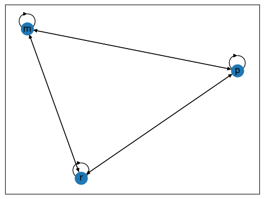
nx.is_strongly_connected(G1) #checking if above graph is strongly connectedTruefig, ax = plt.subplots()
G2 = nx.DiGraph()
G2.add_edges_from([('p', 'p'),
('m', 'p'), ('m', 'm'), ('m', 'r'),
('r', 'p'), ('r', 'm'), ('r', 'r')])
nx.draw_networkx(G2, with_labels = True)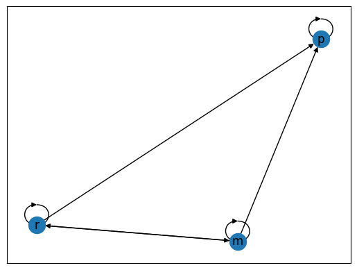
nx.is_strongly_connected(G2) #checking if above graph is strongly connectedFalse41.4Weighted graphs
We now introduce weighted graphs, where weights (numbers) are attached to each edge.
41.4.1International private credit flows by country
To motivate the idea, consider the following figure which shows flows of funds (i.e., loans) between private banks, grouped by country of origin.
Source
Z = ch1_data["adjacency_matrix"]["Z"]
Z_visual= ch1_data["adjacency_matrix"]["Z_visual"]
countries = ch1_data["adjacency_matrix"]["countries"]

G = qbn_io.adjacency_matrix_to_graph(Z_visual, countries, tol=0.03)

centrality = qbn_io.eigenvector_centrality(Z_visual, authority=False)
node_total_exports = qbn_io.node_total_exports(G)
edge_weights = qbn_io.edge_weights(G)

node_pos_dict = nx.circular_layout(G)

node_sizes = qbn_io.normalise_weights(node_total_exports,3000)
edge_widths = qbn_io.normalise_weights(edge_weights,10)


node_colors = qbn_io.colorise_weights(centrality)
node_to_color = dict(zip(G.nodes,node_colors))
edge_colors = []
for src,_ in G.edges:
    edge_colors.append(node_to_color[src])

fig, ax = plt.subplots(figsize=(10, 10))
ax.axis('off')

nx.draw_networkx_nodes(G,
                       node_pos_dict,
                       node_color=node_colors,
                       node_size=node_sizes,
                       edgecolors='grey',
                       linewidths=2,
                       alpha=0.4,
                       ax=ax)

nx.draw_networkx_labels(G,
                        node_pos_dict,
                        font_size=12,
                        ax=ax)

nx.draw_networkx_edges(G,
                       node_pos_dict,
                       edge_color=edge_colors,
                       width=edge_widths,
                       arrows=True,
                       arrowsize=20,
                       alpha=0.8,
                       ax=ax,
                       arrowstyle='->',
                       node_size=node_sizes,
                       connectionstyle='arc3,rad=0.15')

plt.show()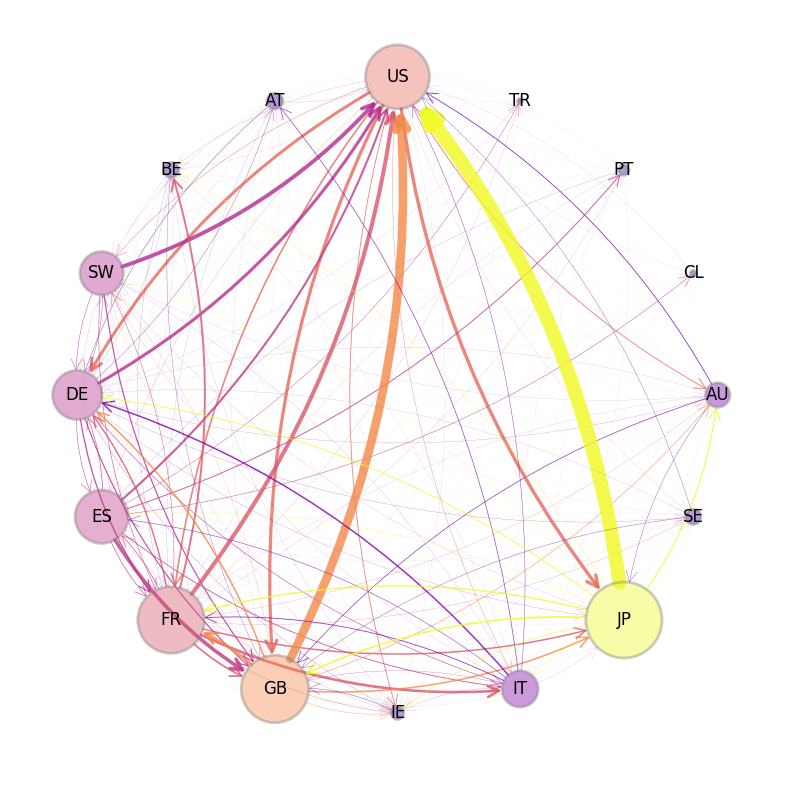
Figure 4:International Credit Network
The country codes are given in the following table
| Code | Country | Code | Country | Code | Country | Code | Country |
|---|---|---|---|---|---|---|---|
| AU | Australia | DE | Germany | CL | Chile | ES | Spain |
| PT | Portugal | FR | France | TR | Turkey | GB | United Kingdom |
| US | United States | IE | Ireland | AT | Austria | IT | Italy |
| BE | Belgium | JP | Japan | SW | Switzerland | SE | Sweden |
An arrow from Japan to the US indicates aggregate claims held by Japanese banks on all US-registered banks, as collected by the Bank of International Settlements (BIS).
The size of each node in the figure is increasing in the total foreign claims of all other nodes on this node.
The widths of the arrows are proportional to the foreign claims they represent.
Notice that, in this network, an edge exists for almost every choice of and (i.e., almost every country in the network).
(In fact, there are even more small arrows, which we have dropped for clarity.)
Hence the existence of an edge from one node to another is not particularly informative.
To understand the network, we need to record not just the existence or absence of a credit flow, but also the size of the flow.
The correct data structure for recording this information is a “weighted directed graph”.
41.4.2Definitions
A weighted directed graph is a directed graph to which we have added a weight function that assigns a positive number to each edge.
The figure above shows one weighted directed graph, where the weights are the size of fund flows.
The following figure shows a weighted directed graph, with arrows representing edges of the induced directed graph.
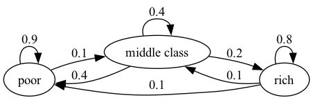
Figure 5:Weighted Poverty Trap
The numbers next to the edges are the weights.
In this case, you can think of the numbers on the arrows as transition probabilities for a household over, say, one year.
We see that a rich household has a 10% chance of becoming poor in one year.
41.5Adjacency matrices
Another way that we can represent weights, which turns out to be very convenient for numerical work, is via a matrix.
The adjacency matrix of a weighted directed graph with nodes , edges and weight function is the matrix
Once the nodes in are enumerated, the weight function and adjacency matrix provide essentially the same information.
For example, with poor, middle, rich mapped to respectively, the adjacency matrix corresponding to the weighted directed graph in Fig. 5 is
In QuantEcon’s DiGraph implementation, weights are recorded via the
keyword weighted:
A = ((0.9, 0.1, 0.0),
     (0.4, 0.4, 0.2),
     (0.1, 0.1, 0.8))
A = np.array(A)
G = qe.DiGraph(A, weighted=True)    # store weights
One of the key points to remember about adjacency matrices is that taking the transpose reverses all the arrows in the associated directed graph.
For example, the following directed graph can be interpreted as a stylized version of a financial network, with nodes as banks and edges showing the flow of funds.
G4 = nx.DiGraph()

G4.add_edges_from([('1','2'),
                   ('2','1'),('2','3'),
                   ('3','4'),
                   ('4','2'),('4','5'),
                   ('5','1'),('5','3'),('5','4')])
pos = nx.circular_layout(G4)

edge_labels={('1','2'): '100',
             ('2','1'): '50', ('2','3'): '200',
             ('3','4'): '100',
             ('4','2'): '500', ('4','5'): '50',
             ('5','1'): '150',('5','3'): '250', ('5','4'): '300'}

nx.draw_networkx(G4, pos, node_color = 'none',node_size = 500)
nx.draw_networkx_edge_labels(G4, pos, edge_labels=edge_labels)
nx.draw_networkx_nodes(G4, pos, linewidths= 0.5, edgecolors = 'black',
                       node_color = 'none',node_size = 500)

plt.show()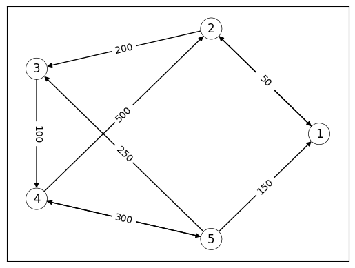
We see that bank 2 extends a loan of size 200 to bank 3.
The corresponding adjacency matrix is
The transpose is
The corresponding network is visualized in the following figure which shows the network of liabilities after the loans have been granted.
Both of these networks (original and transpose) are useful for analyzing financial markets.
G5 = nx.DiGraph()

G5.add_edges_from([('1','2'),('1','5'),
                   ('2','1'),('2','4'),
                   ('3','2'),('3','5'),
                   ('4','3'),('4','5'),
                   ('5','4')])

edge_labels={('1','2'): '50', ('1','5'): '150',
             ('2','1'): '100', ('2','4'): '500',
             ('3','2'): '200', ('3','5'): '250',
             ('4','3'): '100', ('4','5'): '300',
             ('5','4'): '50'}

nx.draw_networkx(G5, pos, node_color = 'none',node_size = 500)
nx.draw_networkx_edge_labels(G5, pos, edge_labels=edge_labels)
nx.draw_networkx_nodes(G5, pos, linewidths= 0.5, edgecolors = 'black',
                       node_color = 'none',node_size = 500)

plt.show()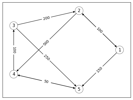
In general, every nonnegative matrix can be viewed as the adjacency matrix of a weighted directed graph.
To build the graph we set and take the edge set to be all such that .
For the weight function we set for all edges .
We call this graph the weighted directed graph induced by .
41.6Properties
Consider a weighted directed graph with adjacency matrix .
Let be element of , the -th power of .
The following result is useful in many applications:
The above result is obvious when and a proof of the general case can be found in Sargent & Stachurski (2022).
Now recall from the eigenvalues lecture that a nonnegative matrix is called irreducible if for each there is an integer such that .
From the preceding theorem, it is not too difficult (see Sargent & Stachurski (2022) for details) to get the next result.
We illustrate the above theorem with a simple example.
Consider the following weighted directed graph.
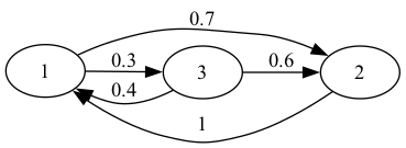
We first create the above network as a Networkx DiGraph object.
G6 = nx.DiGraph()

G6.add_edges_from([('1','2'),('1','3'),
                   ('2','1'),
                   ('3','1'),('3','2')])
Then we construct the associated adjacency matrix A.
A = np.array([[0,0.7,0.3],    # adjacency matrix A
              [1,0,0],
              [0.4,0.6,0]])
Source
def is_irreducible(P):
    n = len(P)
    result = np.zeros((n, n))
    for i in range(n):
        result += np.linalg.matrix_power(P, i)
    return np.all(result > 0)
is_irreducible(A) # check irreducibility of Anp.True_nx.is_strongly_connected(G6) # check connectedness of graphTrue41.7Network centrality
When studying networks of all varieties, a recurring topic is the relative “centrality” or “importance” of different nodes.
Examples include
- ranking of web pages by search engines
- determining the most important bank in a financial network (which one a central bank should rescue if there is a financial crisis)
- determining the most important industrial sector in an economy.
In what follows, a centrality measure associates to each weighted directed graph a vector where the is interpreted as the centrality (or rank) of node .
41.7.1Degree centrality
Two elementary measures of “importance” of a node in a given directed graph are its in-degree and out-degree.
Both of these provide a centrality measure.
In-degree centrality is a vector containing the in-degree of each node in the graph.
Consider the following simple example.
G7 = nx.DiGraph()

G7.add_nodes_from(['1','2','3','4','5','6','7'])

G7.add_edges_from([('1','2'),('1','6'),
                   ('2','1'),('2','4'),
                   ('3','2'),
                   ('4','2'),
                   ('5','3'),('5','4'),
                   ('6','1'),
                   ('7','4'),('7','6')])
pos = nx.planar_layout(G7)

nx.draw_networkx(G7, pos, node_color='none', node_size=500)
nx.draw_networkx_nodes(G7, pos, linewidths=0.5, edgecolors='black',
                       node_color='none',node_size=500)

plt.show()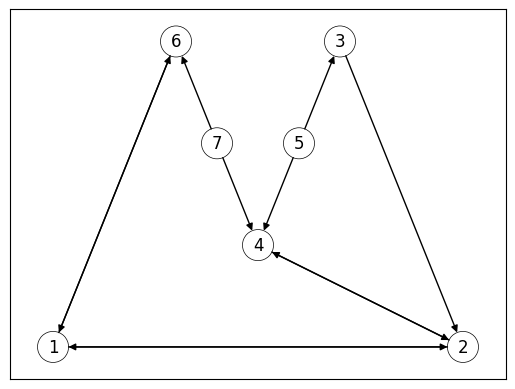
Figure 6:Sample Graph
The following code displays the in-degree centrality of all nodes.
iG7 = [G7.in_degree(v) for v in G7.nodes()]   # computing in-degree centrality

for i, d in enumerate(iG7):
    print(i+1, d)
1 2
2 3
3 1
4 3
5 0
6 2
7 0
Consider the international credit network displayed in Fig. 4.
The following plot displays the in-degree centrality of each country.
D = qbn_io.build_unweighted_matrix(Z)
indegree = D.sum(axis=0)
def centrality_plot_data(countries, centrality_measures):
df = pd.DataFrame({'code': countries,
'centrality':centrality_measures,
'color': qbn_io.colorise_weights(centrality_measures).tolist()
})
return df.sort_values('centrality')fig, ax = plt.subplots()
df = centrality_plot_data(countries, indegree)
ax.bar('code', 'centrality', data=df, color=df["color"], alpha=0.6)
patch = mpatches.Patch(color=None, label='in degree', visible=False)
ax.legend(handles=[patch], fontsize=12, loc="upper left", handlelength=0, frameon=False)
ax.set_ylim((0,20))
plt.show()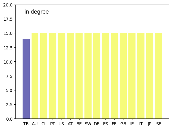
Unfortunately, while in-degree and out-degree centrality are simple to calculate, they are not always informative.
In Fig. 4, an edge exists between almost every node, so the in- or out-degree based centrality ranking fails to effectively separate the countries.
This can be seen in the above graph as well.
Another example is the task of a web search engine, which ranks pages by relevance whenever a user enters a search.
Suppose web page A has twice as many inbound links as page B.
In-degree centrality tells us that page A deserves a higher rank.
But in fact, page A might be less important than page B.
To see why, suppose that the links to A are from pages that receive almost no traffic, while the links to B are from pages that receive very heavy traffic.
In this case, page B probably receives more visitors, which in turn suggests that page B contains more valuable (or entertaining) content.
Thinking about this point suggests that importance might be recursive.
This means that the importance of a given node depends on the importance of other nodes that link to it.
As another example, we can imagine a production network where the importance of a given sector depends on the importance of the sectors that it supplies.
This reverses the order of the previous example: now the importance of a given node depends on the importance of other nodes that it links to.
The next centrality measures will have these recursive features.
41.7.2Eigenvector centrality
Suppose we have a weighted directed graph with adjacency matrix .
For simplicity, we will suppose that the nodes of the graph are just the integers .
Let denote the spectral radius of .
The eigenvector centrality of the graph is defined as the -vector that solves
In other words, is the dominant eigenvector of (the eigenvector of the largest eigenvalue --- see the discussion of the Perron-Frobenius theorem in the eigenvalue lecture.
To better understand (7), we write out the full expression for some element
Note the recursive nature of the definition: the centrality obtained by node is proportional to a sum of the centrality of all nodes, weighted by the rates of flow from into these nodes.
A node is highly ranked if
- there are many edges leaving ,
- these edges have large weights, and
- the edges point to other highly ranked nodes.
Later, when we study demand shocks in production networks, there will be a more concrete interpretation of eigenvector centrality.
We will see that, in production networks, sectors with high eigenvector centrality are important suppliers.
In particular, they are activated by a wide array of demand shocks once orders flow backwards through the network.
To compute eigenvector centrality we can use the following function.
def eigenvector_centrality(A, k=40, authority=False):
    """
    Computes the dominant eigenvector of A. Assumes A is
    primitive and uses the power method.

    """
    A_temp = A.T if authority else A
    n = len(A_temp)
    r = np.max(np.abs(np.linalg.eigvals(A_temp)))
    e = r**(-k) * (np.linalg.matrix_power(A_temp, k) @ np.ones(n))
    return e / np.sum(e)
Let’s compute eigenvector centrality for the graph generated in Fig. 6.
A = nx.to_numpy_array(G7) # compute adjacency matrix of graphe = eigenvector_centrality(A)
n = len(e)
for i in range(n):
print(i+1,e[i])1 0.18580570704268037
2 0.18580570704268037
3 0.11483424225608219
4 0.11483424225608219
5 0.14194292957319637
6 0.11483424225608219
7 0.14194292957319637
While nodes 2 and 4 had the highest in-degree centrality, we can see that nodes 1 and 2 have the highest eigenvector centrality.
Let’s revisit the international credit network in Fig. 4.
eig_central = eigenvector_centrality(Z)fig, ax = plt.subplots()
df = centrality_plot_data(countries, eig_central)
ax.bar('code', 'centrality', data=df, color=df["color"], alpha=0.6)
patch = mpatches.Patch(color=None, visible=False)
ax.legend(handles=[patch], fontsize=12, loc="upper left", handlelength=0, frameon=False)
plt.show()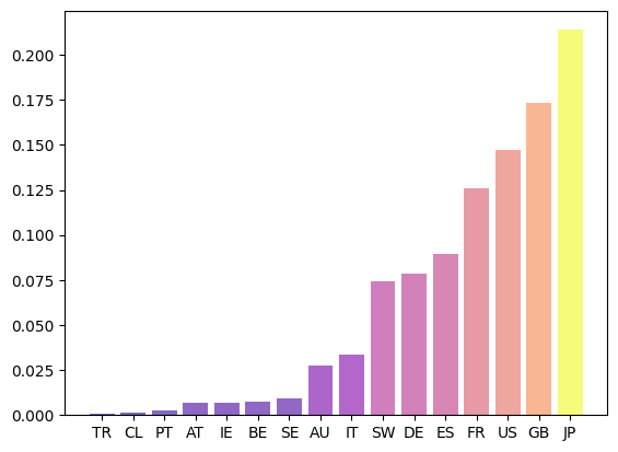
Figure 7:Eigenvector centrality
Countries that are rated highly according to this rank tend to be important players in terms of supply of credit.
Japan takes the highest rank according to this measure, although countries with large financial sectors such as Great Britain and France are not far behind.
The advantage of eigenvector centrality is that it measures a node’s importance while considering the importance of its neighbours.
A variant of eigenvector centrality is at the core of Google’s PageRank algorithm, which is used to rank web pages.
The main principle is that links from important nodes (as measured by degree centrality) are worth more than links from unimportant nodes.
41.7.3Katz centrality
One problem with eigenvector centrality is that might be zero, in which case is not defined.
For this and other reasons, some researchers prefer another measure of centrality for networks called Katz centrality.
Fixing β in , the Katz centrality of a weighted directed graph with adjacency matrix is defined as the vector κ that solves
Here β is a parameter that we can choose.
In vector form we can write
where is a column vector of ones.
The intuition behind this centrality measure is similar to that provided for eigenvector centrality: high centrality is conferred on when it is linked to by nodes that themselves have high centrality.
Provided that , Katz centrality is always finite and well-defined because then .
This means that (10) has the unique solution
This follows from the Neumann series theorem.
The parameter β is used to ensure that κ is finite
When , we use as the default for Katz centrality computations.
41.7.4Authorities vs hubs
Search engine designers recognize that web pages can be important in two different ways.
Some pages have high hub centrality, meaning that they link to valuable sources of information (e.g., news aggregation sites).
Other pages have high authority centrality, meaning that they contain valuable information, as indicated by the number and significance of incoming links (e.g., websites of respected news organizations).
Similar ideas can and have been applied to economic networks (often using different terminology).
The eigenvector centrality and Katz centrality measures we discussed above measure hub centrality.
(Nodes have high centrality if they point to other nodes with high centrality.)
If we care more about authority centrality, we can use the same definitions except that we take the transpose of the adjacency matrix.
This works because taking the transpose reverses the direction of the arrows.
(Now nodes will have high centrality if they receive links from other nodes with high centrality.)
For example, the authority-based eigenvector centrality of a weighted directed graph with adjacency matrix is the vector solving
The only difference from the original definition is that is replaced by its transpose.
(Transposes do not affect the spectral radius of a matrix so we wrote instead of .)
Element-by-element, this is given by
We see will be high if many nodes with high authority rankings link to .
The following figurenshows the authority-based eigenvector centrality ranking for the international credit network shown in Fig. 4.
ecentral_authority = eigenvector_centrality(Z, authority=True)fig, ax = plt.subplots()
df = centrality_plot_data(countries, ecentral_authority)
ax.bar('code', 'centrality', data=df, color=df["color"], alpha=0.6)
patch = mpatches.Patch(color=None, visible=False)
ax.legend(handles=[patch], fontsize=12, loc="upper left", handlelength=0, frameon=False)
plt.show()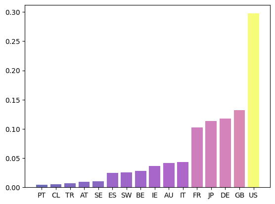
Figure 8:Eigenvector authority
Highly ranked countries are those that attract large inflows of credit, or credit inflows from other major players.
In this case the US clearly dominates the rankings as a target of interbank credit.
41.8Further reading
We apply the ideas discussed in this lecture to:
Textbooks on economic and social networks include Jackson (2010), Easley et al. (2010), Borgatti et al. (2018), Sargent & Stachurski (2022) and Goyal (2023).
Within the realm of network science, the texts by Newman (2018), Menczer et al. (2020) and Coscia (2021) are excellent.
41.9Exercises
Solution to Exercise 1
Reflexivity:
Trivially, .
Thus, .
Symmetry: Suppose,
and .
By definition, this implies .
Transitivity:
Suppose, and
This implies, and and also and .
Thus, we can conclude and .
Which means .
Solution to Exercise 2
# First, let's plot the given graph

G = nx.DiGraph()

G.add_nodes_from(np.arange(8))  # adding nodes

G.add_edges_from([(0,1),(0,3),       # adding edges
                  (1,0),
                  (2,4),
                  (3,2),(3,4),(3,7),
                  (4,3),
                  (5,4),(5,6),
                  (6,3),(6,5),
                  (7,0)])

nx.draw_networkx(G, pos=nx.circular_layout(G), node_color='gray', node_size=500, with_labels=True)

plt.show()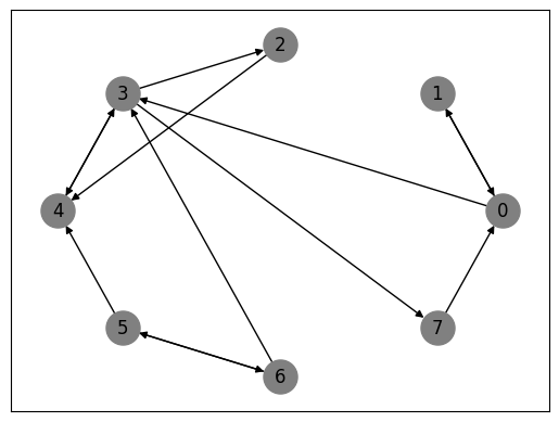
A = nx.to_numpy_array(G)      #find adjacency matrix associated with G

A
array([[0., 1., 0., 1., 0., 0., 0., 0.],
[1., 0., 0., 0., 0., 0., 0., 0.],
[0., 0., 0., 0., 1., 0., 0., 0.],
[0., 0., 1., 0., 1., 0., 0., 1.],
[0., 0., 0., 1., 0., 0., 0., 0.],
[0., 0., 0., 0., 1., 0., 1., 0.],
[0., 0., 0., 1., 0., 1., 0., 0.],
[1., 0., 0., 0., 0., 0., 0., 0.]])oG = [G.out_degree(v) for v in G.nodes()] # computing in-degree centrality
for i, d in enumerate(oG):
print(i, d)0 2
1 1
2 1
3 3
4 1
5 2
6 2
7 1
e = eigenvector_centrality(A)   # computing eigenvector centrality
n = len(e)

for i in range(n):
    print(i+1, e[i])
1 0.1458980838002507
2 0.09016989800748738
3 0.055728056024793506
4 0.14589810100962303
5 0.09016994824024989
6 0.1803397955498566
7 0.20162621936025152
8 0.09016989800748738
Solution to Exercise 3
def is_accessible(G,i,j):
    A = nx.to_numpy_array(G)
    n = len(A)
    result = np.zeros((n, n))
    for i in range(n):
        result += np.linalg.matrix_power(A, i)
    if result[i,j]>0:
        return True
    else:
        return False
G = nx.DiGraph()
G.add_nodes_from(np.arange(8)) # adding nodes
G.add_edges_from([(0,1),(0,3), # adding edges
(1,0),
(2,4),
(3,2),(3,4),(3,7),
(4,3),
(5,4),(5,6),
(6,3),(6,5),
(7,0)])is_accessible(G, 2, 1)Trueis_accessible(G, 3, 6)False- Sargent, T. J., & Stachurski, J. (2022). Economic Networks: Theory and Computation. arXiv Preprint arXiv:2203.11972.
- Jackson, M. O. (2010). Social and economic networks. Princeton university press.
- Easley, D., Kleinberg, J., & others. (2010). Networks, crowds, and markets (Vol. 8). Cambridge university press Cambridge.
- Borgatti, S. P., Everett, M. G., & Johnson, J. C. (2018). Analyzing social networks. Sage.
- Goyal, S. (2023). Networks: An economics approach. MIT Press.
- Newman, M. (2018). Networks. Oxford university press.
- Menczer, F., Fortunato, S., & Davis, C. A. (2020). A first course in network science. Cambridge University Press.
- Coscia, M. (2021). The atlas for the aspiring network scientist. arXiv Preprint arXiv:2101.00863.

Creative Commons License – This work is licensed under a Creative Commons Attribution-ShareAlike 4.0 International.