16. Eigenvalues and Eigenvectors
16.1Overview
Eigenvalues and eigenvectors are a relatively advanced topic in linear algebra.
At the same time, these concepts are extremely useful for
- economic modeling (especially dynamics!)
- statistics
- some parts of applied mathematics
- machine learning
- and many other fields of science.
In this lecture we explain the basics of eigenvalues and eigenvectors and introduce the Neumann Series Lemma.
We assume in this lecture that students are familiar with matrices and understand the basics of matrix algebra.
We will use the following imports:
import matplotlib.pyplot as plt
import numpy as np
from numpy.linalg import matrix_power
from matplotlib.lines import Line2D
from matplotlib.patches import FancyArrowPatch
from mpl_toolkits.mplot3d import proj3d16.2Matrices as transformations
Let’s start by discussing an important concept concerning matrices.
16.2.1Mapping vectors to vectors
One way to think about a matrix is as a rectangular collection of numbers.
Another way to think about a matrix is as a map (i.e., as a function) that transforms vectors to new vectors.
To understand the second point of view, suppose we multiply an matrix with an column vector to obtain an column vector :
If we fix and consider different choices of , we can understand as a map transforming to .
Because is , it transforms -vectors to -vectors.
We can write this formally as .
You might argue that if is a function then we should write rather than but the second notation is more conventional.
16.2.2Square matrices
Let’s restrict our discussion to square matrices.
In the above discussion, this means that and maps to itself.
This means is an matrix that maps (or “transforms”) a vector in to a new vector also in .
Let’s visualize this using Python:
A = np.array([[2,  1],
              [-1, 1]])
from math import sqrt
fig, ax = plt.subplots()
# Set the axes through the origin
for spine in ['left', 'bottom']:
ax.spines[spine].set_position('zero')
for spine in ['right', 'top']:
ax.spines[spine].set_color('none')
ax.set(xlim=(-2, 6), ylim=(-2, 4), aspect=1)
vecs = ((1, 3), (5, 2))
c = ['r', 'black']
for i, v in enumerate(vecs):
ax.annotate('', xy=v, xytext=(0, 0),
arrowprops=dict(color=c[i],
shrink=0,
alpha=0.7,
width=0.5))
ax.text(0.2 + 1, 0.2 + 3, 'x=$(1,3)$')
ax.text(0.2 + 5, 0.2 + 2, 'Ax=$(5,2)$')
ax.annotate('', xy=(sqrt(10/29) * 5, sqrt(10/29) * 2), xytext=(0, 0),
arrowprops=dict(color='purple',
shrink=0,
alpha=0.7,
width=0.5))
ax.annotate('', xy=(1, 2/5), xytext=(1/3, 1),
arrowprops={'arrowstyle': '->',
'connectionstyle': 'arc3,rad=-0.3'},
horizontalalignment='center')
ax.text(0.8, 0.8, f'θ', fontsize=14)
plt.show()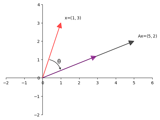
One way to understand this transformation is that
- first rotates by some angle θ and
- then scales it by some scalar γ to obtain the image of .
16.3Types of transformations
Let’s examine some standard transformations we can perform with matrices.
Below we visualize transformations by thinking of vectors as points instead of arrows.
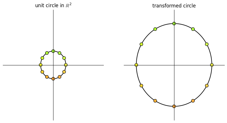
We consider how a given matrix transforms
- a grid of points and
- a set of points located on the unit circle in .
To build the transformations we will use two functions, called grid_transform and circle_transform.
Each of these functions visualizes the actions of a given matrix .
Source
def colorizer(x, y):
r = min(1, 1-y/3)
g = min(1, 1+y/3)
b = 1/4 + x/16
return (r, g, b)
def grid_transform(A=np.array([[1, -1], [1, 1]])):
xvals = np.linspace(-4, 4, 9)
yvals = np.linspace(-3, 3, 7)
xygrid = np.column_stack([[x, y] for x in xvals for y in yvals])
uvgrid = A @ xygrid
colors = list(map(colorizer, xygrid[0], xygrid[1]))
fig, ax = plt.subplots(1, 2, figsize=(10, 5))
for axes in ax:
axes.set(xlim=(-11, 11), ylim=(-11, 11))
axes.set_xticks([])
axes.set_yticks([])
for spine in ['left', 'bottom']:
axes.spines[spine].set_position('zero')
for spine in ['right', 'top']:
axes.spines[spine].set_color('none')
# Plot x-y grid points
ax[0].scatter(xygrid[0], xygrid[1], s=36, c=colors, edgecolor="none")
# ax[0].grid(True)
# ax[0].axis("equal")
ax[0].set_title("points $x_1, x_2, \cdots, x_k$")
# Plot transformed grid points
ax[1].scatter(uvgrid[0], uvgrid[1], s=36, c=colors, edgecolor="none")
# ax[1].grid(True)
# ax[1].axis("equal")
ax[1].set_title("points $Ax_1, Ax_2, \cdots, Ax_k$")
plt.show()
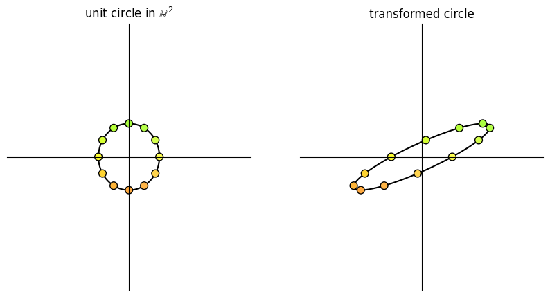
def circle_transform(A=np.array([[-1, 2], [0, 1]])):
fig, ax = plt.subplots(1, 2, figsize=(10, 5))
for axes in ax:
axes.set(xlim=(-4, 4), ylim=(-4, 4))
axes.set_xticks([])
axes.set_yticks([])
for spine in ['left', 'bottom']:
axes.spines[spine].set_position('zero')
for spine in ['right', 'top']:
axes.spines[spine].set_color('none')
θ = np.linspace(0, 2 * np.pi, 150)
r = 1
θ_1 = np.empty(12)
for i in range(12):
θ_1[i] = 2 * np.pi * (i/12)
x = r * np.cos(θ)
y = r * np.sin(θ)
a = r * np.cos(θ_1)
b = r * np.sin(θ_1)
a_1 = a.reshape(1, -1)
b_1 = b.reshape(1, -1)
colors = list(map(colorizer, a, b))
ax[0].plot(x, y, color='black', zorder=1)
ax[0].scatter(a_1, b_1, c=colors, alpha=1, s=60,
edgecolors='black', zorder=2)
ax[0].set_title(r"unit circle in $\mathbb{R}^2$")
x1 = x.reshape(1, -1)
y1 = y.reshape(1, -1)
ab = np.concatenate((a_1, b_1), axis=0)
transformed_ab = A @ ab
transformed_circle_input = np.concatenate((x1, y1), axis=0)
transformed_circle = A @ transformed_circle_input
ax[1].plot(transformed_circle[0, :],
transformed_circle[1, :], color='black', zorder=1)
ax[1].scatter(transformed_ab[0, :], transformed_ab[1:,],
color=colors, alpha=1, s=60, edgecolors='black', zorder=2)
ax[1].set_title("transformed circle")
plt.show()16.3.1Scaling
A matrix of the form
scales vectors across the x-axis by a factor α and along the y-axis by a factor β.
Here we illustrate a simple example where .
A = np.array([[3, 0],  # scaling by 3 in both directions
              [0, 3]])
grid_transform(A)
circle_transform(A)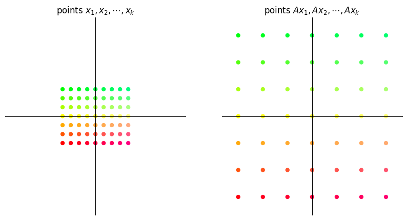
16.3.2Shearing
A “shear” matrix of the form
stretches vectors along the x-axis by an amount proportional to the y-coordinate of a point.
A = np.array([[1, 2],     # shear along x-axis
              [0, 1]])
grid_transform(A)
circle_transform(A)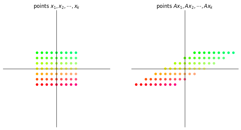
16.3.3Rotation
A matrix of the form
is called a rotation matrix.
This matrix rotates vectors clockwise by an angle θ.
θ = np.pi/4  # 45 degree clockwise rotation
A = np.array([[np.cos(θ), np.sin(θ)],
              [-np.sin(θ), np.cos(θ)]])
grid_transform(A)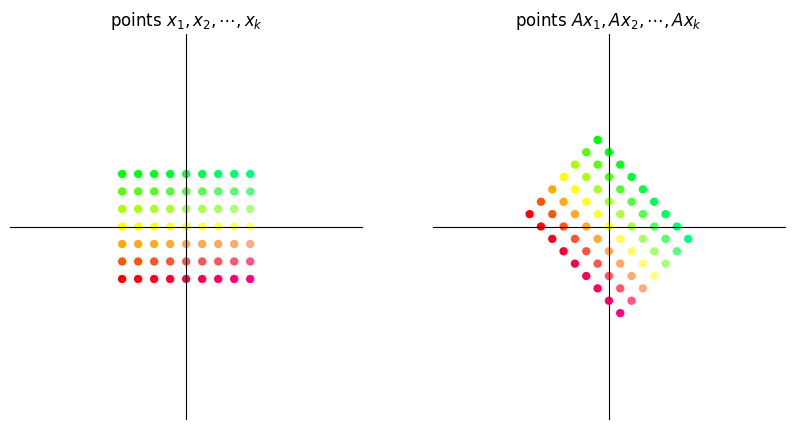
A = np.column_stack([[0, 1], [1, 0]])
grid_transform(A)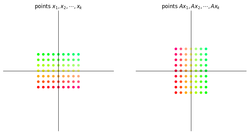
More examples of common transition matrices can be found here.
16.4Matrix multiplication as composition
Since matrices act as functions that transform one vector to another, we can apply the concept of function composition to matrices as well.
16.4.1Linear compositions
Consider the two matrices
What will the output be when we try to obtain for some vector ?
We can observe that applying the transformation on the vector is the same as first applying on and then applying on the vector .
Thus the matrix product is the composition of the matrix transformations and
This means first apply transformation and then transformation .
When we matrix multiply an matrix with an matrix the obtained matrix product is an matrix .
Thus, if and are transformations such that and , then transforms to .
Viewing matrix multiplication as composition of maps helps us understand why, under matrix multiplication, is generally not equal to .
(After all, when we compose functions, the order usually matters.)
16.4.2Examples
Let be the clockwise rotation matrix given by and let be a shear matrix along the x-axis given by .
We will visualize how a grid of points changes when we apply the transformation and then compare it with the transformation .
Source
def grid_composition_transform(A=np.array([[1, -1], [1, 1]]),
                               B=np.array([[1, -1], [1, 1]])):
    xvals = np.linspace(-4, 4, 9)
    yvals = np.linspace(-3, 3, 7)
    xygrid = np.column_stack([[x, y] for x in xvals for y in yvals])
    uvgrid = B @ xygrid
    abgrid = A @ uvgrid

    colors = list(map(colorizer, xygrid[0], xygrid[1]))

    fig, ax = plt.subplots(1, 3, figsize=(15, 5))

    for axes in ax:
        axes.set(xlim=(-12, 12), ylim=(-12, 12))
        axes.set_xticks([])
        axes.set_yticks([])
        for spine in ['left', 'bottom']:
            axes.spines[spine].set_position('zero')
        for spine in ['right', 'top']:
            axes.spines[spine].set_color('none')

    # Plot grid points
    ax[0].scatter(xygrid[0], xygrid[1], s=36, c=colors, edgecolor="none")
    ax[0].set_title(r"points $x_1, x_2, \cdots, x_k$")

    # Plot intermediate grid points
    ax[1].scatter(uvgrid[0], uvgrid[1], s=36, c=colors, edgecolor="none")
    ax[1].set_title(r"points $Bx_1, Bx_2, \cdots, Bx_k$")

    # Plot transformed grid points
    ax[2].scatter(abgrid[0], abgrid[1], s=36, c=colors, edgecolor="none")
    ax[2].set_title(r"points $ABx_1, ABx_2, \cdots, ABx_k$")

    plt.show()
A = np.array([[0, 1], # 90 degree clockwise rotation
[-1, 0]])
B = np.array([[1, 2], # shear along x-axis
[0, 1]])16.4.2.1Shear then rotate
grid_composition_transform(A, B) # transformation AB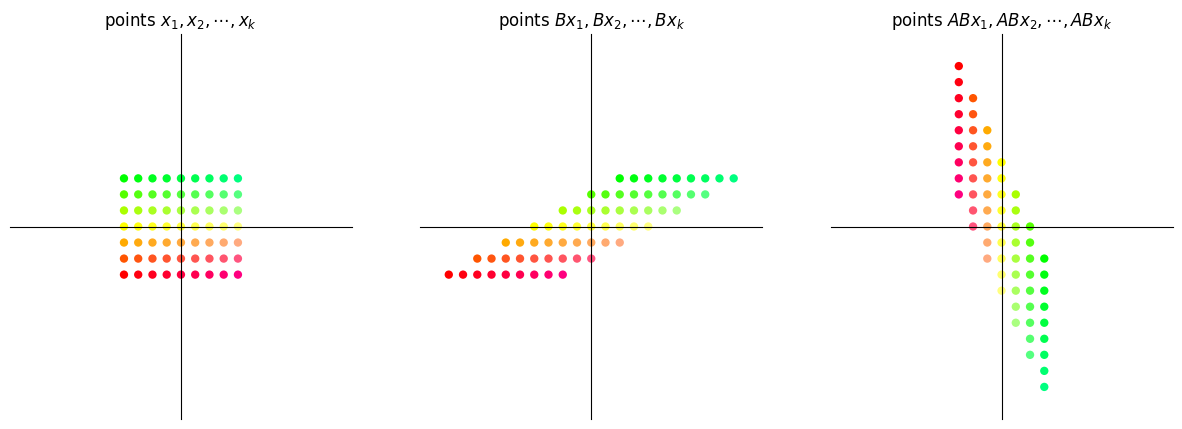
16.4.2.2Rotate then shear
grid_composition_transform(B,A) # transformation BA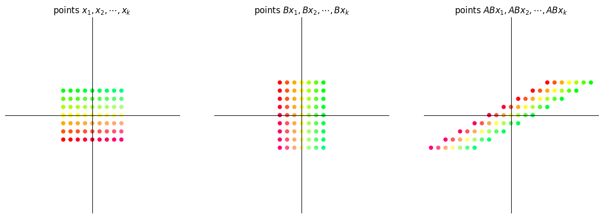
It is evident that the transformation is not the same as the transformation .
16.5Iterating on a fixed map
In economics (and especially in dynamic modeling), we are often interested in analyzing behavior where we repeatedly apply a fixed matrix.
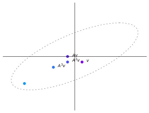
For example, given a vector and a matrix , we are interested in studying the sequence
Let’s first see examples of a sequence of iterates under different maps .
def plot_series(A, v, n):

    B = np.array([[1, -1],
                  [1, 0]])

    fig, ax = plt.subplots()

    ax.set(xlim=(-4, 4), ylim=(-4, 4))
    ax.set_xticks([])
    ax.set_yticks([])
    for spine in ['left', 'bottom']:
        ax.spines[spine].set_position('zero')
    for spine in ['right', 'top']:
        ax.spines[spine].set_color('none')

    θ = np.linspace(0, 2 * np.pi, 150)
    r = 2.5
    x = r * np.cos(θ)
    y = r * np.sin(θ)
    x1 = x.reshape(1, -1)
    y1 = y.reshape(1, -1)
    xy = np.concatenate((x1, y1), axis=0)

    ellipse = B @ xy
    ax.plot(ellipse[0, :], ellipse[1, :], color='black',
            linestyle=(0, (5, 10)), linewidth=0.5)

    # Initialize holder for trajectories
    colors = plt.cm.rainbow(np.linspace(0, 1, 20))

    for i in range(n):
        iteration = matrix_power(A, i) @ v
        v1 = iteration[0]
        v2 = iteration[1]
        ax.scatter(v1, v2, color=colors[i])
        if i == 0:
            ax.text(v1+0.25, v2, f'$v$')
        elif i == 1:
            ax.text(v1+0.25, v2, f'$Av$')
        elif 1 < i < 4:
            ax.text(v1+0.25, v2, f'$A^{i}v$')
    plt.show()
A = np.array([[sqrt(3) + 1, -2],
[1, sqrt(3) - 1]])
A = (1/(2*sqrt(2))) * A
v = (-3, -3)
n = 12
plot_series(A, v, n)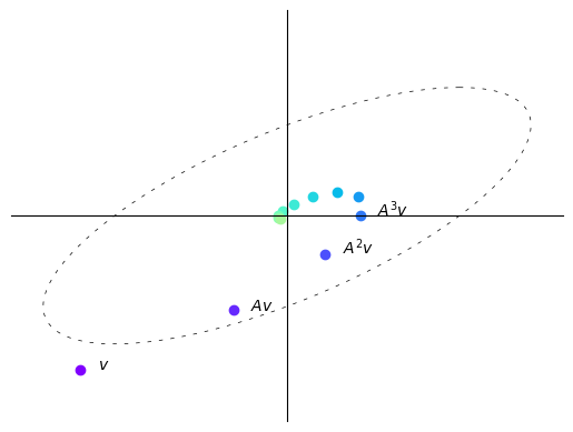
Here with each iteration the vectors get shorter, i.e., move closer to the origin.
In this case, repeatedly multiplying a vector by makes the vector “spiral in”.
B = np.array([[sqrt(3) + 1, -2],
              [1, sqrt(3) - 1]])
B = (1/2) * B
v = (2.5, 0)
n = 12

plot_series(B, v, n)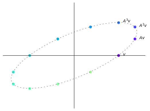
Here with each iteration vectors do not tend to get longer or shorter.
In this case, repeatedly multiplying a vector by simply “rotates it around an ellipse”.
B = np.array([[sqrt(3) + 1, -2],
              [1, sqrt(3) - 1]])
B = (1/sqrt(2)) * B
v = (-1, -0.25)
n = 6

plot_series(B, v, n)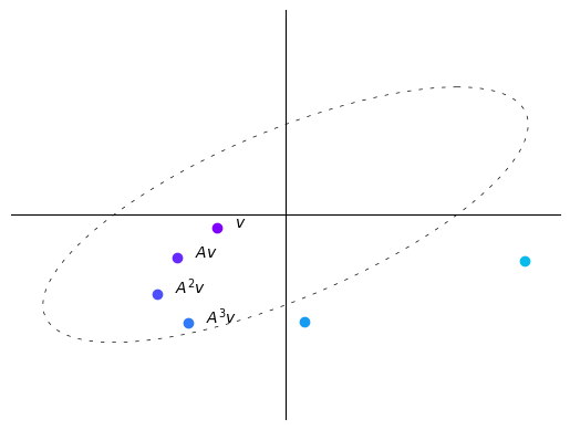
Here with each iteration vectors tend to get longer, i.e., farther from the origin.
In this case, repeatedly multiplying a vector by makes the vector “spiral out”.
We thus observe that the sequence behaves differently depending on the map itself.
We now discuss the property of A that determines this behavior.
16.6Eigenvalues
In this section we introduce the notions of eigenvalues and eigenvectors.
16.6.1Definitions
Let be an square matrix.
If λ is scalar and is a non-zero -vector such that
Then we say that λ is an eigenvalue of , and is the corresponding eigenvector.
Thus, an eigenvector of is a nonzero vector such that when the map is applied, is merely scaled.
The next figure shows two eigenvectors (blue arrows) and their images under (red arrows).
As expected, the image of each is just a scaled version of the original
from numpy.linalg import eig

A = [[1, 2],
     [2, 1]]
A = np.array(A)
evals, evecs = eig(A)
evecs = evecs[:, 0], evecs[:, 1]

fig, ax = plt.subplots(figsize=(10, 8))
# Set the axes through the origin
for spine in ['left', 'bottom']:
    ax.spines[spine].set_position('zero')
for spine in ['right', 'top']:
    ax.spines[spine].set_color('none')
# ax.grid(alpha=0.4)

xmin, xmax = -3, 3
ymin, ymax = -3, 3
ax.set(xlim=(xmin, xmax), ylim=(ymin, ymax))

# Plot each eigenvector
for v in evecs:
    ax.annotate('', xy=v, xytext=(0, 0),
                arrowprops=dict(facecolor='blue',
                shrink=0,
                alpha=0.6,
                width=0.5))

# Plot the image of each eigenvector
for v in evecs:
    v = A @ v
    ax.annotate('', xy=v, xytext=(0, 0),
                arrowprops=dict(facecolor='red',
                shrink=0,
                alpha=0.6,
                width=0.5))

# Plot the lines they run through
x = np.linspace(xmin, xmax, 3)
for v in evecs:
    a = v[1] / v[0]
    ax.plot(x, a * x, 'b-', lw=0.4)

plt.show()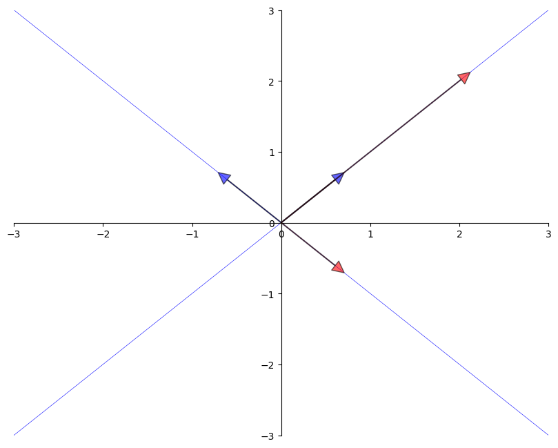
16.6.2Complex values
So far our definition of eigenvalues and eigenvectors seems straightforward.
There is one complication we haven’t mentioned yet:
When solving ,
- λ is allowed to be a complex number and
- is allowed to be an -vector of complex numbers.
We will see some examples below.
16.6.3Some mathematical details
We note some mathematical details for more advanced readers.
(Other readers can skip to the next section.)
The eigenvalue equation is equivalent to .
This equation has a nonzero solution only when the columns of are linearly dependent.
This in turn is equivalent to stating the determinant is zero.
Hence, to find all eigenvalues, we can look for λ such that the determinant of is zero.
This problem can be expressed as one of solving for the roots of a polynomial in λ of degree .
This in turn implies the existence of solutions in the complex plane, although some might be repeated.
16.6.4Facts
Some nice facts about the eigenvalues of a square matrix are as follows:
- the determinant of equals the product of the eigenvalues
- the trace of (the sum of the elements on the principal diagonal) equals the sum of the eigenvalues
- if is symmetric, then all of its eigenvalues are real
- if is invertible and are its eigenvalues, then the eigenvalues of are .
A corollary of the last statement is that a matrix is invertible if and only if all its eigenvalues are nonzero.
16.6.5Computation
Using NumPy, we can solve for the eigenvalues and eigenvectors of a matrix as follows
from numpy.linalg import eig

A = ((1, 2),
     (2, 1))

A = np.array(A)
evals, evecs = eig(A)
evals  # eigenvalues
array([ 3., -1.])evecs # eigenvectorsarray([[ 0.70710678, -0.70710678],
[ 0.70710678, 0.70710678]])Note that the columns of evecs are the eigenvectors.
Since any scalar multiple of an eigenvector is an eigenvector with the same
eigenvalue (which can be verified), the eig routine normalizes the length of each eigenvector
to one.
The eigenvectors and eigenvalues of a map determine how a vector is transformed when we repeatedly multiply by .
This is discussed further later.
16.7The Neumann Series Lemma
In this section we present a famous result about series of matrices that has many applications in economics.
16.7.1Scalar series
Here’s a fundamental result about series:
If is a number and , then
For a one-dimensional linear equation where x is unknown we can thus conclude that the solution is given by:
16.7.2Matrix series
A generalization of this idea exists in the matrix setting.
Consider the system of equations where is an square matrix and and are both column vectors in .
Using matrix algebra we can conclude that the solution to this system of equations will be given by:
What guarantees the existence of a unique vector that satisfies (15)?
The following is a fundamental result in functional analysis that generalizes (13) to a multivariate case.
We can see the Neumann Series Lemma in action in the following example.
A = np.array([[0.4, 0.1],
              [0.7, 0.2]])

evals, evecs = eig(A)   # finding eigenvalues and eigenvectors

r = max(abs(λ) for λ in evals)    # compute spectral radius
print(r)
0.5828427124746189
The spectral radius obtained is less than 1.
Thus, we can apply the Neumann Series Lemma to find .
I = np.identity(2)  # 2 x 2 identity matrix
B = I - A
B_inverse = np.linalg.inv(B) # direct inverse methodA_sum = np.zeros((2, 2)) # power series sum of A
A_power = I
for i in range(50):
A_sum += A_power
A_power = A_power @ ALet’s check equality between the sum and the inverse methods.
np.allclose(A_sum, B_inverse)TrueAlthough we truncate the infinite sum at , both methods give us the same result which illustrates the result of the Neumann Series Lemma.
16.8Exercises
Solution to Exercise 1
Here is one solution.
We start by looking into the distance between the eigenvector approximation and the true eigenvector.
# Define a matrix A
A = np.array([[1, 0, 3],
              [0, 2, 0],
              [3, 0, 1]])

num_iters = 20

# Define a random starting vector b
b = np.random.rand(A.shape[1])

# Get the leading eigenvector of matrix A
eigenvector = np.linalg.eig(A)[1][:, 0]

errors = []
res = []

# Power iteration loop
for i in range(num_iters):
    # Multiply b by A
    b = A @ b
    # Normalize b
    b = b / np.linalg.norm(b)
    # Append b to the list of eigenvector approximations
    res.append(b)
    err = np.linalg.norm(np.array(b)
                         - eigenvector)
    errors.append(err)

greatest_eigenvalue = np.dot(A @ b, b) / np.dot(b, b)
print(f'The approximated greatest absolute eigenvalue is \
        {greatest_eigenvalue:.2f}')
print('The real eigenvalue is', np.linalg.eig(A)[0])

# Plot the eigenvector approximations for each iteration
plt.figure(figsize=(10, 6))
plt.xlabel('iterations')
plt.ylabel('error')
_ = plt.plot(errors)
The approximated greatest absolute eigenvalue is 4.00
The real eigenvalue is [ 4. -2. 2.]
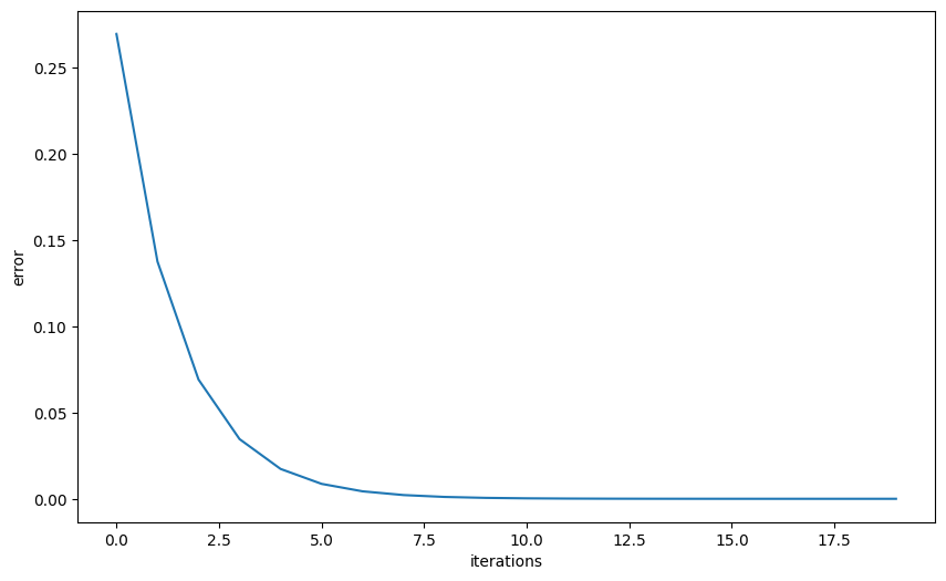
Figure 1:Power iteration
Then we can look at the trajectory of the eigenvector approximation.
# Set up the figure and axis for 3D plot
fig = plt.figure()
ax = fig.add_subplot(111, projection='3d')

# Plot the eigenvectors
ax.scatter(eigenvector[0],
           eigenvector[1],
           eigenvector[2],
           color='r', s=80)

for i, vec in enumerate(res):
    ax.scatter(vec[0], vec[1], vec[2],
               color='b',
               alpha=(i+1)/(num_iters+1),
               s=80)

ax.set_xlabel('x')
ax.set_ylabel('y')
ax.set_zlabel('z')
ax.tick_params(axis='both', which='major', labelsize=7)

points = [plt.Line2D([0], [0], linestyle='none',
                     c=i, marker='o') for i in ['r', 'b']]
ax.legend(points, ['actual eigenvector',
                   r'approximated eigenvector ($b_k$)'])
ax.set_box_aspect(aspect=None, zoom=0.8)

plt.show()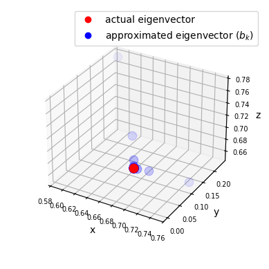
Figure 2:Power iteration trajectory
Solution to Exercise 2
A = np.array([[1, 2],
              [1, 1]])
v = (0.4, -0.4)
n = 11

# Compute eigenvectors and eigenvalues
eigenvalues, eigenvectors = np.linalg.eig(A)

print(f'eigenvalues:\n {eigenvalues}')
print(f'eigenvectors:\n {eigenvectors}')

plot_series(A, v, n)
eigenvalues:
[ 2.41421356 -0.41421356]
eigenvectors:
[[ 0.81649658 -0.81649658]
[ 0.57735027 0.57735027]]
The result seems to converge to the eigenvector of with the largest eigenvalue.
Let’s use a vector field to visualize the transformation brought by A.
(This is a more advanced topic in linear algebra, please step ahead if you are comfortable with the math.)
# Create a grid of points
x, y = np.meshgrid(np.linspace(-5, 5, 15),
                   np.linspace(-5, 5, 20))

# Apply the matrix A to each point in the vector field
vec_field = np.stack([x, y])
u, v = np.tensordot(A, vec_field, axes=1)

# Plot the transformed vector field
c = plt.streamplot(x, y, u - x, v - y,
                   density=1, linewidth=None, color='#A23BEC')
c.lines.set_alpha(0.5)
c.arrows.set_alpha(0.5)

# Draw eigenvectors
origin = np.zeros((2, len(eigenvectors)))
parameters = {'color': ['b', 'g'], 'angles': 'xy',
              'scale_units': 'xy', 'scale': 0.1, 'width': 0.01}
plt.quiver(*origin, eigenvectors[0],
           eigenvectors[1], **parameters)
plt.quiver(*origin, - eigenvectors[0],
           - eigenvectors[1], **parameters)

colors = ['b', 'g']
lines = [Line2D([0], [0], color=c, linewidth=3) for c in colors]
labels = ["2.4 eigenspace", "0.4 eigenspace"]
plt.legend(lines, labels, loc='center left',
           bbox_to_anchor=(1, 0.5))

plt.xlabel("x")
plt.ylabel("y")
plt.grid()
plt.gca().set_aspect('equal', adjustable='box')
plt.show()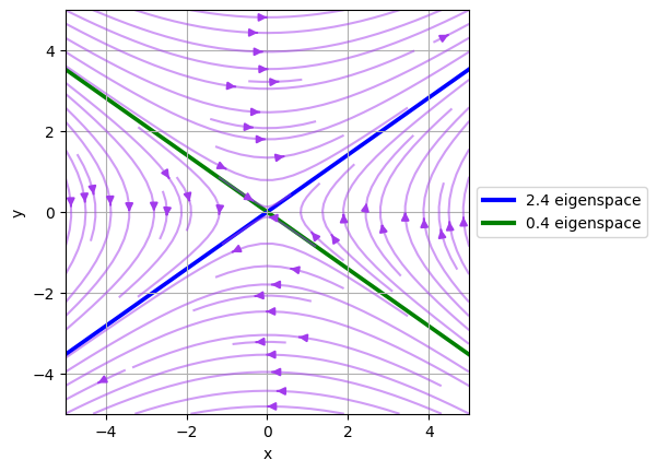
Figure 3:Convergence towards eigenvectors
Note that the vector field converges to the eigenvector of with the largest eigenvalue and diverges from the eigenvector of with the smallest eigenvalue.
In fact, the eigenvectors are also the directions in which the matrix stretches or shrinks the space.
Specifically, the eigenvector with the largest eigenvalue is the direction in which the matrix stretches the space the most.
We will see more intriguing examples in the following exercise.
Solution to Exercise 3
Here is one solution
figure, ax = plt.subplots(1, 3, figsize=(15, 5))
A = np.array([[sqrt(3) + 1, -2],
              [1, sqrt(3) - 1]])
A = (1/(2*sqrt(2))) * A

B = np.array([[sqrt(3) + 1, -2],
              [1, sqrt(3) - 1]])
B = (1/2) * B

C = np.array([[sqrt(3) + 1, -2],
              [1, sqrt(3) - 1]])
C = (1/sqrt(2)) * C

examples = [A, B, C]

for i, example in enumerate(examples):
    M = example

    # Compute right eigenvectors and eigenvalues
    eigenvalues, eigenvectors = np.linalg.eig(M)
    print(f'Example {i+1}:\n')
    print(f'eigenvalues:\n {eigenvalues}')
    print(f'eigenvectors:\n {eigenvectors}\n')

    eigenvalues_real = eigenvalues.real
    eigenvectors_real = eigenvectors.real

    # Create a grid of points
    x, y = np.meshgrid(np.linspace(-20, 20, 15),
                       np.linspace(-20, 20, 20))

    # Apply the matrix A to each point in the vector field
    vec_field = np.stack([x, y])
    u, v = np.tensordot(M, vec_field, axes=1)

    # Plot the transformed vector field
    c = ax[i].streamplot(x, y, u - x, v - y, density=1,
                         linewidth=None, color='#A23BEC')
    c.lines.set_alpha(0.5)
    c.arrows.set_alpha(0.5)

    # Draw eigenvectors
    parameters = {'color': ['b', 'g'], 'angles': 'xy',
                  'scale_units': 'xy', 'scale': 1,
                  'width': 0.01, 'alpha': 0.5}
    origin = np.zeros((2, len(eigenvectors)))
    ax[i].quiver(*origin, eigenvectors_real[0],
                 eigenvectors_real[1], **parameters)
    ax[i].quiver(*origin,
                 - eigenvectors_real[0],
                 - eigenvectors_real[1],
                 **parameters)

    ax[i].set_xlabel("x-axis")
    ax[i].set_ylabel("y-axis")
    ax[i].grid()
    ax[i].set_aspect('equal', adjustable='box')

plt.show()
Example 1:
eigenvalues:
[0.61237244+0.35355339j 0.61237244-0.35355339j]
eigenvectors:
[[0.81649658+0.j 0.81649658-0.j ]
[0.40824829-0.40824829j 0.40824829+0.40824829j]]
Example 2:

eigenvalues:
 [0.8660254+0.5j 0.8660254-0.5j]
eigenvectors:
 [[0.81649658+0.j         0.81649658-0.j        ]
 [0.40824829-0.40824829j 0.40824829+0.40824829j]]
Example 3:

eigenvalues:
 [1.22474487+0.70710678j 1.22474487-0.70710678j]
eigenvectors:
 [[0.81649658+0.j         0.81649658-0.j        ]
 [0.40824829-0.40824829j 0.40824829+0.40824829j]]
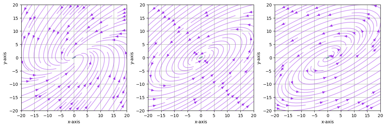
Figure 4:Vector fields of the three matrices
The vector fields explain why we observed the trajectories of the vector multiplied by iteratively before.
The pattern demonstrated here is because we have complex eigenvalues and eigenvectors.
We can plot the complex plane for one of the matrices using Arrow3D class retrieved from stackoverflow.
class Arrow3D(FancyArrowPatch):
    def __init__(self, xs, ys, zs, *args, **kwargs):
        super().__init__((0, 0), (0, 0), *args, **kwargs)
        self._verts3d = xs, ys, zs

    def do_3d_projection(self):
        xs3d, ys3d, zs3d = self._verts3d
        xs, ys, zs = proj3d.proj_transform(xs3d, ys3d, zs3d,
                                           self.axes.M)
        self.set_positions((0.1*xs[0], 0.1*ys[0]),
                           (0.1*xs[1], 0.1*ys[1]))

        return np.min(zs)


eigenvalues, eigenvectors = np.linalg.eig(A)

# Create meshgrid for vector field
x, y = np.meshgrid(np.linspace(-2, 2, 15),
                   np.linspace(-2, 2, 15))

# Calculate vector field (real and imaginary parts)
u_real = A[0][0] * x + A[0][1] * y
v_real = A[1][0] * x + A[1][1] * y
u_imag = np.zeros_like(x)
v_imag = np.zeros_like(y)

# Create 3D figure
fig = plt.figure()
ax = fig.add_subplot(111, projection='3d')
vlength = np.linalg.norm(eigenvectors)
ax.quiver(x, y, u_imag, u_real-x, v_real-y, v_imag-u_imag,
          colors='b', alpha=0.3, length=.2,
          arrow_length_ratio=0.01)

arrow_prop_dict = dict(mutation_scale=5,
                       arrowstyle='-|>', shrinkA=0, shrinkB=0)

# Plot 3D eigenvectors
for c, i in zip(['b', 'g'], [0, 1]):
    a = Arrow3D([0, eigenvectors[0][i].real],
                [0, eigenvectors[1][i].real],
                [0, eigenvectors[1][i].imag],
                color=c, **arrow_prop_dict)
    ax.add_artist(a)

# Set axis labels and title
ax.set_xlabel('x')
ax.set_ylabel('y')
ax.set_zlabel('Im')
ax.set_box_aspect(aspect=None, zoom=0.8)

plt.draw()
plt.show()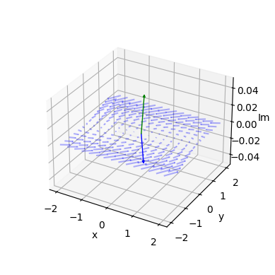
Figure 5:3D plot of the vector field

Creative Commons License – This work is licensed under a Creative Commons Attribution-ShareAlike 4.0 International.