44. Simple Linear Regression Model
import numpy as np
import pandas as pd
import matplotlib.pyplot as plt
The simple regression model estimates the relationship between two variables and
where represents the error between the line of best fit and the sample values for given .
Our goal is to choose values for α and β to build a line of “best” fit for some data that is available for variables and .
Let us consider a simple dataset of 10 observations for variables and :
| 1 | 2000 | 32 |
| 2 | 1000 | 21 |
| 3 | 1500 | 24 |
| 4 | 2500 | 35 |
| 5 | 500 | 10 |
| 6 | 900 | 11 |
| 7 | 1100 | 22 |
| 8 | 1500 | 21 |
| 9 | 1800 | 27 |
| 10 | 250 | 2 |
Let us think about as sales for an ice-cream cart, while is a variable that records the day’s temperature in Celsius.
x = [32, 21, 24, 35, 10, 11, 22, 21, 27, 2]
y = [2000,1000,1500,2500,500,900,1100,1500,1800, 250]
df = pd.DataFrame([x,y]).T
df.columns = ['X', 'Y']
dfWe can use a scatter plot of the data to see the relationship between (ice-cream sales in dollars ($'s)) and (degrees Celsius).
ax = df.plot(
    x='X',
    y='Y',
    kind='scatter',
    ylabel='Ice-cream sales ($\'s)',
    xlabel='Degrees celcius'
)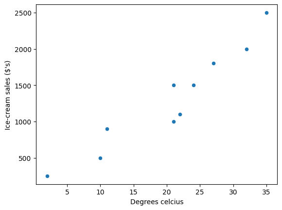
Figure 1:Scatter plot
as you can see the data suggests that more ice-cream is typically sold on hotter days.
To build a linear model of the data we need to choose values for α and β that represents a line of “best” fit such that
Let’s start with and
α = 5
β = 10
df['Y_hat'] = α + β * df['X']
fig, ax = plt.subplots()
ax = df.plot(x='X',y='Y', kind='scatter', ax=ax)
ax = df.plot(x='X',y='Y_hat', kind='line', ax=ax)
plt.show()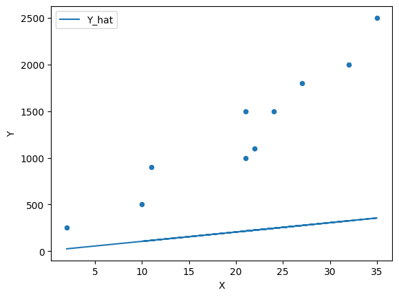
Figure 2:Scatter plot with a line of fit
We can see that this model does a poor job of estimating the relationship.
We can continue to guess and iterate towards a line of “best” fit by adjusting the parameters
β = 100
df['Y_hat'] = α + β * df['X']
fig, ax = plt.subplots()
ax = df.plot(x='X',y='Y', kind='scatter', ax=ax)
ax = df.plot(x='X',y='Y_hat', kind='line', ax=ax)
plt.show()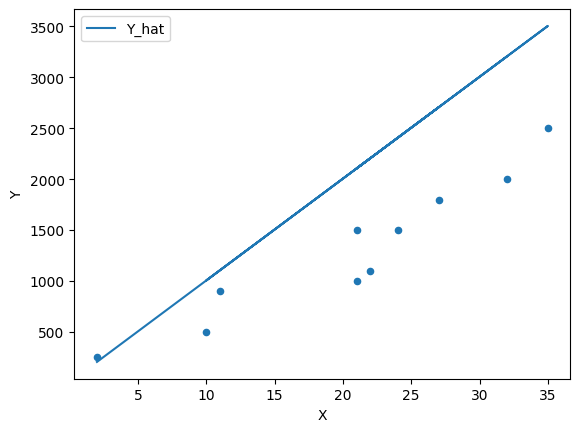
Figure 3:Scatter plot with a line of fit #2
β = 65
df['Y_hat'] = α + β * df['X']
fig, ax = plt.subplots()
ax = df.plot(x='X',y='Y', kind='scatter', ax=ax)
ax = df.plot(x='X',y='Y_hat', kind='line', ax=ax, color='g')
plt.show()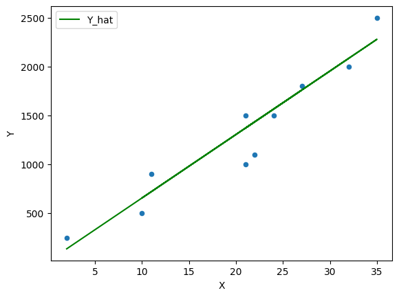
Figure 4:Scatter plot with a line of fit #3
However we need to think about formalizing this guessing process by thinking of this problem as an optimization problem.
Let’s consider the error and define the difference between the observed values and the estimated values which we will call the residuals
df['error'] = df['Y_hat'] - df['Y']dffig, ax = plt.subplots()
ax = df.plot(x='X',y='Y', kind='scatter', ax=ax)
ax = df.plot(x='X',y='Y_hat', kind='line', ax=ax, color='g')
plt.vlines(df['X'], df['Y_hat'], df['Y'], color='r')
plt.show()
Figure 5:Plot of the residuals
The Ordinary Least Squares (OLS) method chooses α and β in such a way that minimizes the sum of the squared residuals (SSR).
Let’s call this a cost function
that we would like to minimize with parameters α and β.
44.1How does error change with respect to α and β
Let us first look at how the total error changes with respect to β (holding the intercept α constant)
We know from the next section the optimal values for α and β are:
β_optimal = 64.38
α_optimal = -14.72
We can then calculate the error for a range of β values
errors = {}
for β in np.arange(20,100,0.5):
    errors[β] = abs((α_optimal + β * df['X']) - df['Y']).sum()
Plotting the error
ax = pd.Series(errors).plot(xlabel='β', ylabel='error')
plt.axvline(β_optimal, color='r');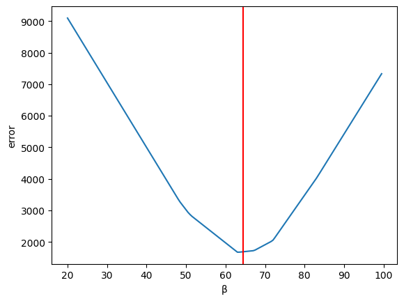
Figure 6:Plotting the error
Now let us vary α (holding β constant)
errors = {}
for α in np.arange(-500,500,5):
    errors[α] = abs((α + β_optimal * df['X']) - df['Y']).sum()
Plotting the error
ax = pd.Series(errors).plot(xlabel='α', ylabel='error')
plt.axvline(α_optimal, color='r');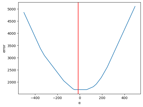
Figure 7:Plotting the error (2)
44.2Calculating optimal values
Now let us use calculus to solve the optimization problem and compute the optimal values for α and β to find the ordinary least squares solution.
First taking the partial derivative with respect to α
and setting it equal to 0
we can remove the constant -2 from the summation by dividing both sides by -2
Now we can split this equation up into the components
The middle term is a straight forward sum from by a constant α
and rearranging terms
We observe that both fractions resolve to the means and
Now let’s take the partial derivative of the cost function with respect to β
and setting it equal to 0
we can again take the constant outside of the summation and divide both sides by -2
which becomes
now substituting for α
and rearranging terms
This can be split into two summations
and solving for β yields
We can now use (12) and (20) to calculate the optimal values for α and β
Calculating β
df = df[['X','Y']].copy()  # Original Data

# Calculate the sample means
x_bar = df['X'].mean()
y_bar = df['Y'].mean()
Now computing across the 10 observations and then summing the numerator and denominator
# Compute the Sums
df['num'] = df['X'] * df['Y'] - y_bar * df['X']
df['den'] = pow(df['X'],2) - x_bar * df['X']
β = df['num'].sum() / df['den'].sum()
print(β)
64.37665782493369
Calculating α
α = y_bar - β * x_bar
print(α)
-14.72148541114052
Now we can plot the OLS solution
df['Y_hat'] = α + β * df['X']
df['error'] = df['Y_hat'] - df['Y']

fig, ax = plt.subplots()
ax = df.plot(x='X',y='Y', kind='scatter', ax=ax)
ax = df.plot(x='X',y='Y_hat', kind='line', ax=ax, color='g')
plt.vlines(df['X'], df['Y_hat'], df['Y'], color='r');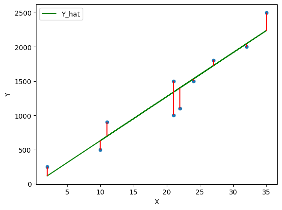
Figure 8:OLS line of best fit

Creative Commons License – This work is licensed under a Creative Commons Attribution-ShareAlike 4.0 International.