21. Heavy-Tailed Distributions
In addition to what’s in Anaconda, this lecture will need the following libraries:
!pip install --upgrade yfinance pandas_datareaderOutput
Requirement already satisfied: yfinance in /opt/hostedtoolcache/Python/3.12.9/x64/lib/python3.12/site-packages (0.2.53)
Collecting pandas_datareader
  Using cached pandas_datareader-0.10.0-py3-none-any.whl.metadata (2.9 kB)
Requirement already satisfied: pandas>=1.3.0 in /opt/hostedtoolcache/Python/3.12.9/x64/lib/python3.12/site-packages (from yfinance) (2.2.3)
Requirement already satisfied: numpy>=1.16.5 in /opt/hostedtoolcache/Python/3.12.9/x64/lib/python3.12/site-packages (from yfinance) (2.1.3)
Requirement already satisfied: requests>=2.31 in /opt/hostedtoolcache/Python/3.12.9/x64/lib/python3.12/site-packages (from yfinance) (2.32.3)
Requirement already satisfied: multitasking>=0.0.7 in /opt/hostedtoolcache/Python/3.12.9/x64/lib/python3.12/site-packages (from yfinance) (0.0.11)
Requirement already satisfied: platformdirs>=2.0.0 in /opt/hostedtoolcache/Python/3.12.9/x64/lib/python3.12/site-packages (from yfinance) (4.3.6)
Requirement already satisfied: pytz>=2022.5 in /opt/hostedtoolcache/Python/3.12.9/x64/lib/python3.12/site-packages (from yfinance) (2025.1)
Requirement already satisfied: frozendict>=2.3.4 in /opt/hostedtoolcache/Python/3.12.9/x64/lib/python3.12/site-packages (from yfinance) (2.4.6)
Requirement already satisfied: peewee>=3.16.2 in /opt/hostedtoolcache/Python/3.12.9/x64/lib/python3.12/site-packages (from yfinance) (3.17.9)
Requirement already satisfied: beautifulsoup4>=4.11.1 in /opt/hostedtoolcache/Python/3.12.9/x64/lib/python3.12/site-packages (from yfinance) (4.13.3)
Collecting lxml (from pandas_datareader)
  Using cached lxml-5.3.1-cp312-cp312-manylinux_2_28_x86_64.whl.metadata (3.7 kB)
Requirement already satisfied: soupsieve>1.2 in /opt/hostedtoolcache/Python/3.12.9/x64/lib/python3.12/site-packages (from beautifulsoup4>=4.11.1->yfinance) (2.6)
Requirement already satisfied: typing-extensions>=4.0.0 in /opt/hostedtoolcache/Python/3.12.9/x64/lib/python3.12/site-packages (from beautifulsoup4>=4.11.1->yfinance) (4.12.2)
Requirement already satisfied: python-dateutil>=2.8.2 in /opt/hostedtoolcache/Python/3.12.9/x64/lib/python3.12/site-packages (from pandas>=1.3.0->yfinance) (2.9.0.post0)
Requirement already satisfied: tzdata>=2022.7 in /opt/hostedtoolcache/Python/3.12.9/x64/lib/python3.12/site-packages (from pandas>=1.3.0->yfinance) (2025.1)
Requirement already satisfied: charset-normalizer<4,>=2 in /opt/hostedtoolcache/Python/3.12.9/x64/lib/python3.12/site-packages (from requests>=2.31->yfinance) (3.4.1)
Requirement already satisfied: idna<4,>=2.5 in /opt/hostedtoolcache/Python/3.12.9/x64/lib/python3.12/site-packages (from requests>=2.31->yfinance) (3.10)
Requirement already satisfied: urllib3<3,>=1.21.1 in /opt/hostedtoolcache/Python/3.12.9/x64/lib/python3.12/site-packages (from requests>=2.31->yfinance) (2.3.0)
Requirement already satisfied: certifi>=2017.4.17 in /opt/hostedtoolcache/Python/3.12.9/x64/lib/python3.12/site-packages (from requests>=2.31->yfinance) (2025.1.31)
Requirement already satisfied: six>=1.5 in /opt/hostedtoolcache/Python/3.12.9/x64/lib/python3.12/site-packages (from python-dateutil>=2.8.2->pandas>=1.3.0->yfinance) (1.17.0)
Using cached pandas_datareader-0.10.0-py3-none-any.whl (109 kB)
Using cached lxml-5.3.1-cp312-cp312-manylinux_2_28_x86_64.whl (5.0 MB)
Installing collected packages: lxml, pandas_datareader
Successfully installed lxml-5.3.1 pandas_datareader-0.10.0
We use the following imports.
import matplotlib.pyplot as plt
import numpy as np
import yfinance as yf
import pandas as pd
import statsmodels.api as sm

from pandas_datareader import wb
from scipy.stats import norm, cauchy
from pandas.plotting import register_matplotlib_converters
register_matplotlib_converters()21.1Overview
Heavy-tailed distributions are a class of distributions that generate “extreme” outcomes.
In the natural sciences (and in more traditional economics courses), heavy-tailed distributions are seen as quite exotic and non-standard.
However, it turns out that heavy-tailed distributions play a crucial role in economics.
In fact many -- if not most -- of the important distributions in economics are heavy-tailed.
In this lecture we explain what heavy tails are and why they are -- or at least why they should be -- central to economic analysis.
21.1.1Introduction: light tails
Most commonly used probability distributions in classical statistics and the natural sciences have “light tails.”
To explain this concept, let’s look first at examples.
We can see this when we plot the density and show a histogram of observations, as with the following code (which assumes and ).
fig, ax = plt.subplots()
X = norm.rvs(size=1_000_000)
ax.hist(X, bins=40, alpha=0.4, label='histogram', density=True)
x_grid = np.linspace(-4, 4, 400)
ax.plot(x_grid, norm.pdf(x_grid), label='density')
ax.legend()
plt.show()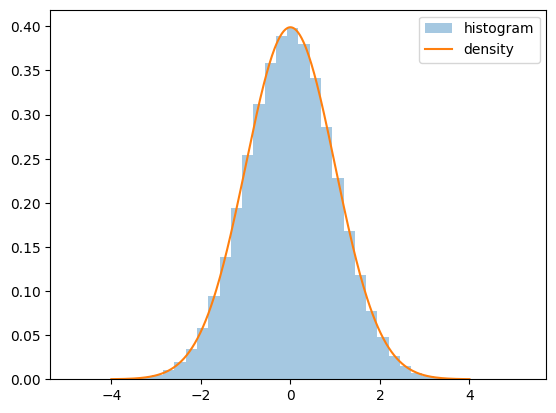
Figure 1:Histogram of observations
Notice how
- the density’s tails converge quickly to zero in both directions and
- even with 1,000,000 draws, we get no very large or very small observations.
We can see the last point more clearly by executing
X.min(), X.max()(np.float64(-4.855770947865966), np.float64(5.2170300601365))Here’s another view of draws from the same distribution:
n = 2000
fig, ax = plt.subplots()
data = norm.rvs(size=n)
ax.plot(list(range(n)), data, linestyle='', marker='o', alpha=0.5, ms=4)
ax.vlines(list(range(n)), 0, data, lw=0.2)
ax.set_ylim(-15, 15)
ax.set_xlabel('$i$')
ax.set_ylabel('$X_i$', rotation=0)
plt.show()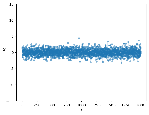
Figure 2:Histogram of observations
We have plotted each individual draw against .
None are very large or very small.
In other words, extreme observations are rare and draws tend not to deviate too much from the mean.
Putting this another way, light-tailed distributions are those that rarely generate extreme values.
(A more formal definition is given below.)
Many statisticians and econometricians use rules of thumb such as “outcomes more than four or five standard deviations from the mean can safely be ignored.”
But this is only true when distributions have light tails.
21.1.2When are light tails valid?
In probability theory and in the real world, many distributions are light-tailed.
For example, human height is light-tailed.
Yes, it’s true that we see some very tall people.
- For example, basketballer Sun Mingming is 2.32 meters tall
But have you ever heard of someone who is 20 meters tall? Or 200? Or 2000?
Have you ever wondered why not?
After all, there are 8 billion people in the world!
In essence, the reason we don’t see such draws is that the distribution of human height has very light tails.
In fact the distribution of human height obeys a bell-shaped curve similar to the normal distribution.
21.1.3Returns on assets
But what about economic data?
Let’s look at some financial data first.
Our aim is to plot the daily change in the price of Amazon (AMZN) stock for the period from 1st January 2015 to 1st July 2022.
This equates to daily returns if we set dividends aside.
The code below produces the desired plot using Yahoo financial data via the yfinance library.
data = yf.download('AMZN', '2015-1-1', '2022-7-1')Output
YF.download() has changed argument auto_adjust default to True
s = data['Close']
r = s.pct_change()

fig, ax = plt.subplots()

ax.plot(r, linestyle='', marker='o', alpha=0.5, ms=4)
ax.vlines(r.index, 0, r.values, lw=0.2)
ax.set_ylabel('returns', fontsize=12)
ax.set_xlabel('date', fontsize=12)

plt.show()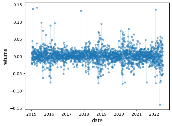
Figure 3:Daily Amazon returns
This data looks different to the draws from the normal distribution we saw above.
Several of observations are quite extreme.
We get a similar picture if we look at other assets, such as Bitcoin
data = yf.download('BTC-USD', '2015-1-1', '2022-7-1')Output
s = data['Close']
r = s.pct_change()

fig, ax = plt.subplots()

ax.plot(r, linestyle='', marker='o', alpha=0.5, ms=4)
ax.vlines(r.index, 0, r.values, lw=0.2)
ax.set_ylabel('returns', fontsize=12)
ax.set_xlabel('date', fontsize=12)

plt.show()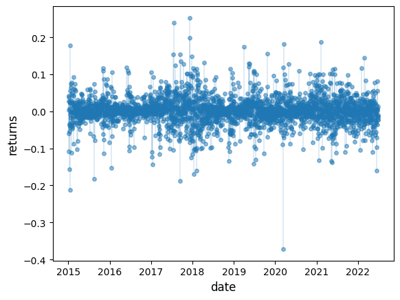
Figure 4:Daily Bitcoin returns
The histogram also looks different to the histogram of the normal distribution:
r = np.random.standard_t(df=5, size=1000)

fig, ax = plt.subplots()
ax.hist(r, bins=60, alpha=0.4, label='bitcoin returns', density=True)

xmin, xmax = plt.xlim()
x = np.linspace(xmin, xmax, 100)
p = norm.pdf(x, np.mean(r), np.std(r))
ax.plot(x, p, linewidth=2, label='normal distribution')

ax.set_xlabel('returns', fontsize=12)
ax.legend()

plt.show()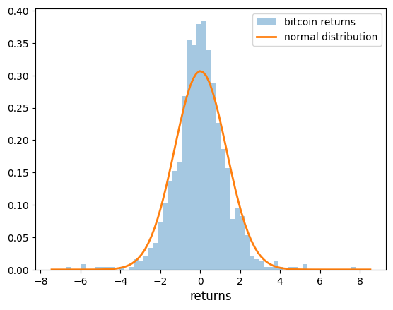
Figure 5:Histogram (normal vs bitcoin returns)
If we look at higher frequency returns data (e.g., tick-by-tick), we often see even more extreme observations.
See, for example, Mandelbrot (1963) or Rachev (2003).
21.1.4Other data
The data we have just seen is said to be “heavy-tailed”.
With heavy-tailed distributions, extreme outcomes occur relatively frequently.
Later in this lecture, we examine heavy tails in these distributions.
21.1.5Why should we care?
Heavy tails are common in economic data but does that mean they are important?
The answer to this question is affirmative!
When distributions are heavy-tailed, we need to think carefully about issues like
- diversification and risk
- forecasting
- taxation (across a heavy-tailed income distribution), etc.
We return to these points below.
21.2Visual comparisons
In this section, we will introduce important concepts such as the Pareto distribution, Counter CDFs, and Power laws, which aid in recognizing heavy-tailed distributions.
Later we will provide a mathematical definition of the difference between light and heavy tails.
But for now let’s do some visual comparisons to help us build intuition on the difference between these two types of distributions.
21.2.1Simulations
The figure below shows a simulation.
The top two subfigures each show 120 independent draws from the normal distribution, which is light-tailed.
The bottom subfigure shows 120 independent draws from the Cauchy distribution, which is heavy-tailed.
n = 120
np.random.seed(11)

fig, axes = plt.subplots(3, 1, figsize=(6, 12))

for ax in axes:
    ax.set_ylim((-120, 120))

s_vals = 2, 12

for ax, s in zip(axes[:2], s_vals):
    data = np.random.randn(n) * s
    ax.plot(list(range(n)), data, linestyle='', marker='o', alpha=0.5, ms=4)
    ax.vlines(list(range(n)), 0, data, lw=0.2)
    ax.set_title(fr"draws from $N(0, \sigma^2)$ with $\sigma = {s}$", fontsize=11)

ax = axes[2]
distribution = cauchy()
data = distribution.rvs(n)
ax.plot(list(range(n)), data, linestyle='', marker='o', alpha=0.5, ms=4)
ax.vlines(list(range(n)), 0, data, lw=0.2)
ax.set_title(f"draws from the Cauchy distribution", fontsize=11)

plt.subplots_adjust(hspace=0.25)

plt.show()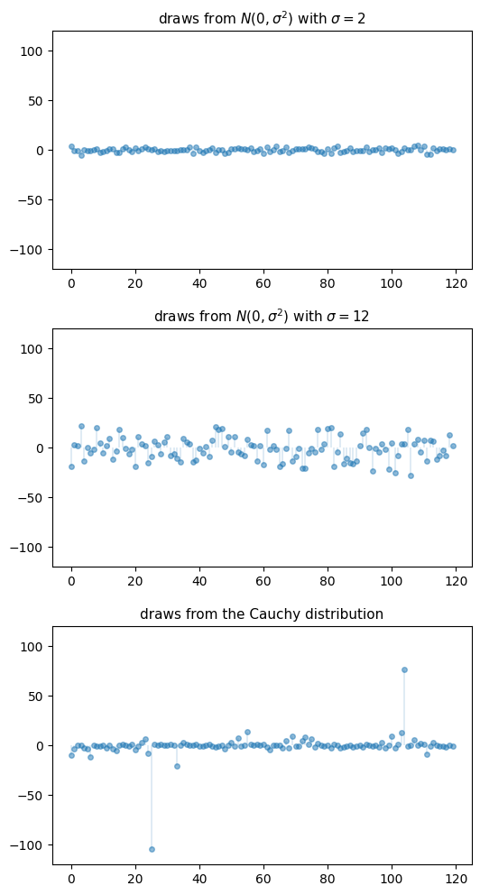
Figure 6:Draws from normal and Cauchy distributions
In the top subfigure, the standard deviation of the normal distribution is 2, and the draws are clustered around the mean.
In the middle subfigure, the standard deviation is increased to 12 and, as expected, the amount of dispersion rises.
The bottom subfigure, with the Cauchy draws, shows a different pattern: tight clustering around the mean for the great majority of observations, combined with a few sudden large deviations from the mean.
This is typical of a heavy-tailed distribution.
21.2.2Nonnegative distributions
Let’s compare some distributions that only take nonnegative values.
One is the exponential distribution, which we discussed in our lecture on probability and distributions.
The exponential distribution is a light-tailed distribution.
Here are some draws from the exponential distribution.
n = 120
np.random.seed(11)

fig, ax = plt.subplots()
ax.set_ylim((0, 50))

data = np.random.exponential(size=n)
ax.plot(list(range(n)), data, linestyle='', marker='o', alpha=0.5, ms=4)
ax.vlines(list(range(n)), 0, data, lw=0.2)

plt.show()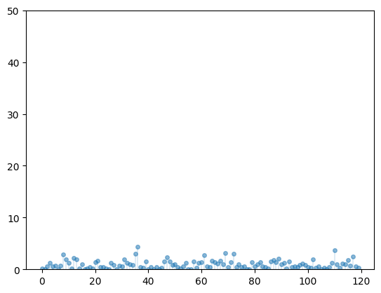
Figure 7:Draws of exponential distribution
Another nonnegative distribution is the Pareto distribution.
If has the Pareto distribution, then there are positive constants and α such that
The parameter α is called the tail index and is called the minimum.
The Pareto distribution is a heavy-tailed distribution.
One way that the Pareto distribution arises is as the exponential of an exponential random variable.
In particular, if is exponentially distributed with rate parameter α, then
is Pareto-distributed with minimum and tail index α.
Here are some draws from the Pareto distribution with tail index 1 and minimum 1.
n = 120
np.random.seed(11)

fig, ax = plt.subplots()
ax.set_ylim((0, 80))
exponential_data = np.random.exponential(size=n)
pareto_data = np.exp(exponential_data)
ax.plot(list(range(n)), pareto_data, linestyle='', marker='o', alpha=0.5, ms=4)
ax.vlines(list(range(n)), 0, pareto_data, lw=0.2)

plt.show()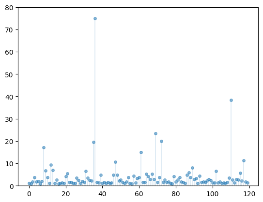
Figure 8:Draws from Pareto distribution
Notice how extreme outcomes are more common.
21.2.3Counter CDFs
For nonnegative random variables, one way to visualize the difference between light and heavy tails is to look at the counter CDF (CCDF).
For a random variable with CDF , the CCDF is the function
(Some authors call the “survival” function.)
The CCDF shows how fast the upper tail goes to zero as .
If is exponentially distributed with rate parameter α, then the CCDF is
This function goes to zero relatively quickly as gets large.
The standard Pareto distribution, where , has CCDF
This function goes to zero as , but much slower than .
Solution to Exercise 1
Letting and be defined as above, letting be exponentially distributed with rate parameter α, and letting , we have
Here’s a plot that illustrates how goes to zero faster than .
x = np.linspace(1.5, 100, 1000)
fig, ax = plt.subplots()
alpha = 1.0
ax.plot(x, np.exp(- alpha * x), label='exponential', alpha=0.8)
ax.plot(x, x**(- alpha), label='Pareto', alpha=0.8)
ax.set_xlabel('X value')
ax.set_ylabel('CCDF')
ax.legend()
plt.show()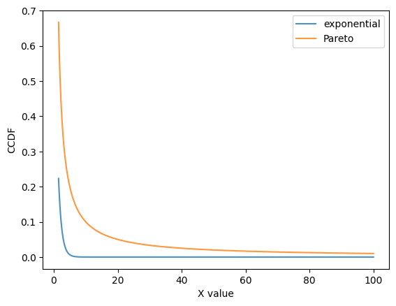
Figure 9:Pareto and exponential distribution comparison
Here’s a log-log plot of the same functions, which makes visual comparison easier.
fig, ax = plt.subplots()
alpha = 1.0
ax.loglog(x, np.exp(- alpha * x), label='exponential', alpha=0.8)
ax.loglog(x, x**(- alpha), label='Pareto', alpha=0.8)
ax.set_xlabel('log value')
ax.set_ylabel('log prob')
ax.legend()
plt.show()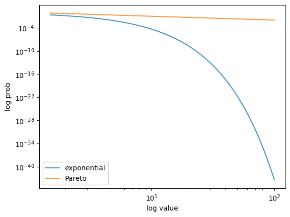
Figure 10:Pareto and exponential distribution comparison (log-log)
In the log-log plot, the Pareto CCDF is linear, while the exponential one is concave.
This idea is often used to separate light- and heavy-tailed distributions in visualisations --- we return to this point below.
21.2.4Empirical CCDFs
The sample counterpart of the CCDF function is the empirical CCDF.
Given a sample , the empirical CCDF is given by
Thus, shows the fraction of the sample that exceeds .
def eccdf(x, data):
    "Simple empirical CCDF function."
    return np.mean(data > x)
Here’s a figure containing some empirical CCDFs from simulated data.
# Parameters and grid
x_grid = np.linspace(1, 1000, 1000)
sample_size = 1000
np.random.seed(13)
z = np.random.randn(sample_size)

# Draws
data_exp = np.random.exponential(size=sample_size)
data_logn = np.exp(z)
data_pareto = np.exp(np.random.exponential(size=sample_size))

data_list = [data_exp, data_logn, data_pareto]

# Build figure
fig, axes = plt.subplots(3, 1, figsize=(6, 8))
axes = axes.flatten()
labels = ['exponential', 'lognormal', 'Pareto']

for data, label, ax in zip(data_list, labels, axes):

    ax.loglog(x_grid, [eccdf(x, data) for x in x_grid],
        'o', markersize=3.0, alpha=0.5, label=label)
    ax.set_xlabel("log value")
    ax.set_ylabel("log prob")

    ax.legend()


fig.subplots_adjust(hspace=0.4)

plt.show()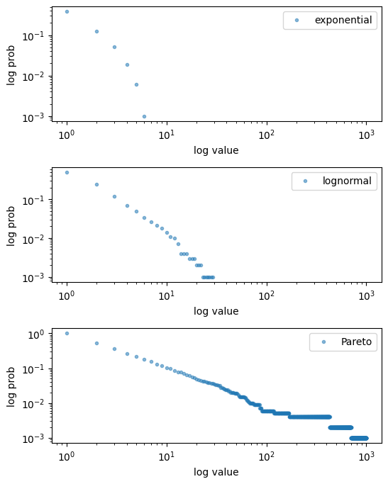
Figure 11:Empirical CCDFs
As with the CCDF, the empirical CCDF from the Pareto distributions is approximately linear in a log-log plot.
We will use this idea below when we look at real data.
21.2.4.1Q-Q Plots
We can also use a qq plot to do a visual comparison between two probability distributions.
The statsmodels package provides a convenient qqplot function that, by default, compares sample data to the quintiles of the normal distribution.
If the data is drawn from a normal distribution, the plot would look like:
data_normal = np.random.normal(size=sample_size)
sm.qqplot(data_normal, line='45')
plt.show()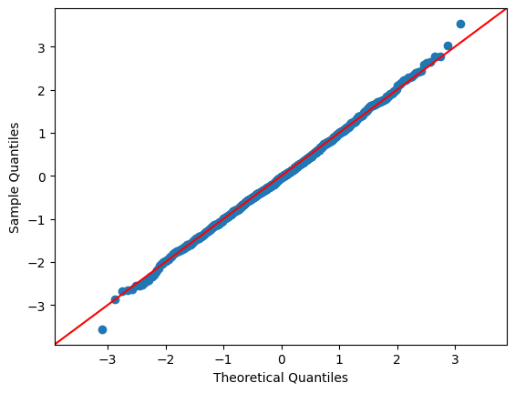
We can now compare this with the exponential, log-normal, and Pareto distributions
# Build figure
fig, axes = plt.subplots(1, 3, figsize=(12, 4))
axes = axes.flatten()
labels = ['exponential', 'lognormal', 'Pareto']
for data, label, ax in zip(data_list, labels, axes):
    sm.qqplot(data, line='45', ax=ax, )
    ax.set_title(label)
plt.tight_layout()
plt.show()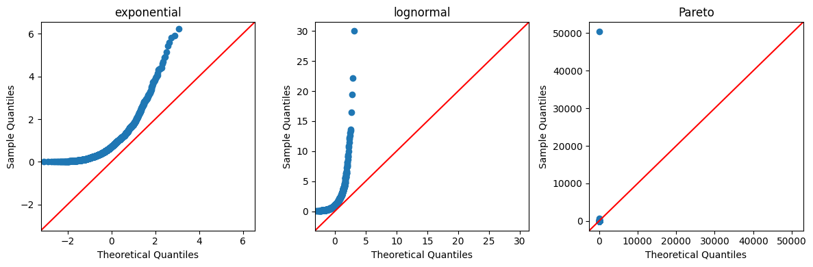
21.2.5Power laws
One specific class of heavy-tailed distributions has been found repeatedly in economic and social phenomena: the class of so-called power laws.
A random variable is said to have a power law if, for some ,
We can write this more mathematically as
It is also common to say that a random variable with this property has a Pareto tail with tail index α.
Notice that every Pareto distribution with tail index α has a Pareto tail with tail index α.
We can think of power laws as a generalization of Pareto distributions.
They are distributions that resemble Pareto distributions in their upper right tail.
Another way to think of power laws is a set of distributions with a specific kind of (very) heavy tail.
21.3Heavy tails in economic cross-sections
As mentioned above, heavy tails are pervasive in economic data.
In fact power laws seem to be very common as well.
We now illustrate this by showing the empirical CCDF of heavy tails.
All plots are in log-log, so that a power law shows up as a linear log-log plot, at least in the upper tail.
We hide the code that generates the figures, which is somewhat complex, but readers are of course welcome to explore the code (perhaps after examining the figures).
Source
def empirical_ccdf(data,
                   ax,
                   aw=None,   # weights
                   label=None,
                   xlabel=None,
                   add_reg_line=False,
                   title=None):
    """
    Take data vector and return prob values for plotting.
    Upgraded empirical_ccdf
    """
    y_vals = np.empty_like(data, dtype='float64')
    p_vals = np.empty_like(data, dtype='float64')
    n = len(data)
    if aw is None:
        for i, d in enumerate(data):
            # record fraction of sample above d
            y_vals[i] = np.sum(data >= d) / n
            p_vals[i] = np.sum(data == d) / n
    else:
        fw = np.empty_like(aw, dtype='float64')
        for i, a in enumerate(aw):
            fw[i] = a / np.sum(aw)
        pdf = lambda x: np.interp(x, data, fw)
        data = np.sort(data)
        j = 0
        for i, d in enumerate(data):
            j += pdf(d)
            y_vals[i] = 1- j

    x, y = np.log(data), np.log(y_vals)

    results = sm.OLS(y, sm.add_constant(x)).fit()
    b, a = results.params

    kwargs = [('alpha', 0.3)]
    if label:
        kwargs.append(('label', label))
    kwargs = dict(kwargs)

    ax.scatter(x, y, **kwargs)
    if add_reg_line:
        ax.plot(x, x * a + b, 'k-', alpha=0.6, label=f"slope = ${a: 1.2f}$")
    if not xlabel:
        xlabel='log value'
    ax.set_xlabel(xlabel, fontsize=12)
    ax.set_ylabel("log prob", fontsize=12)

    if label:
        ax.legend(loc='lower left', fontsize=12)

    if title:
        ax.set_title(title)

    return np.log(data), y_vals, p_vals
Source
def extract_wb(varlist=['NY.GDP.MKTP.CD'],
               c='all_countries',
               s=1900,
               e=2021,
               varnames=None):
    if c == "all_countries":
        # Keep countries only (no aggregated regions)
        countries = wb.get_countries()
        countries_name = countries[countries['region'] != 'Aggregates']['name'].values
        c = "all"

    df = wb.download(indicator=varlist, country=c, start=s, end=e).stack().unstack(0).reset_index()
    df = df.drop(['level_1'], axis=1).transpose()
    if varnames is not None:
        df.columns = varnames
        df = df[1:]

    df1 =df[df.index.isin(countries_name)]
return df121.3.1Firm size
Here is a plot of the firm size distribution for the largest 500 firms in 2020 taken from Forbes Global 2000.
Source
df_fs = pd.read_csv('https://media.githubusercontent.com/media/QuantEcon/high_dim_data/main/cross_section/forbes-global2000.csv')
df_fs = df_fs[['Country', 'Sales', 'Profits', 'Assets', 'Market Value']]
fig, ax = plt.subplots(figsize=(6.4, 3.5))

label="firm size (market value)"
top = 500 # set the cutting for top
d = df_fs.sort_values('Market Value', ascending=False)
empirical_ccdf(np.asarray(d['Market Value'])[:top], ax, label=label, add_reg_line=True)

plt.show()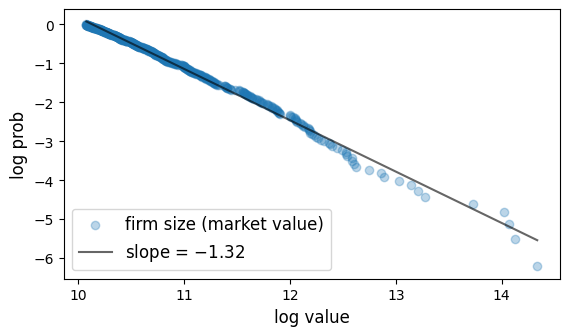
Figure 12:Firm size distribution
21.3.2City size
Here are plots of the city size distribution for the US and Brazil in 2023 from the World Population Review.
The size is measured by population.
Source
# import population data of cities in 2023 United States and 2023 Brazil from world population review
df_cs_us = pd.read_csv('https://media.githubusercontent.com/media/QuantEcon/high_dim_data/main/cross_section/cities_us.csv')
df_cs_br = pd.read_csv('https://media.githubusercontent.com/media/QuantEcon/high_dim_data/main/cross_section/cities_brazil.csv')

fig, axes = plt.subplots(1, 2, figsize=(8.8, 3.6))

empirical_ccdf(np.asarray(df_cs_us["pop2023"]), axes[0], label="US", add_reg_line=True)
empirical_ccdf(np.asarray(df_cs_br['pop2023']), axes[1], label="Brazil", add_reg_line=True)

plt.show()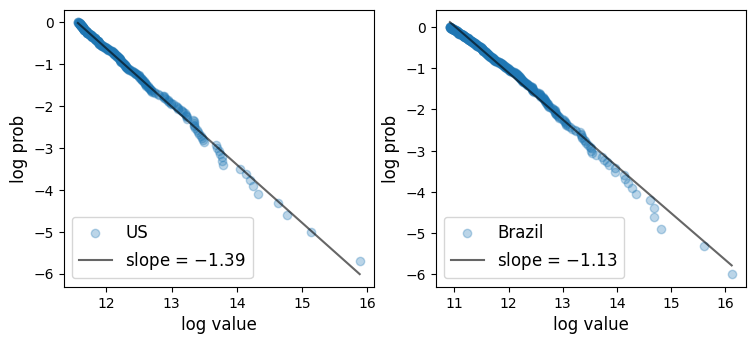
Figure 13:City size distribution
21.3.3Wealth
Here is a plot of the upper tail (top 500) of the wealth distribution.
The data is from the Forbes Billionaires list in 2020.
Source
df_w = pd.read_csv('https://media.githubusercontent.com/media/QuantEcon/high_dim_data/main/cross_section/forbes-billionaires.csv')
df_w = df_w[['country', 'realTimeWorth', 'realTimeRank']].dropna()
df_w = df_w.astype({'realTimeRank': int})
df_w = df_w.sort_values('realTimeRank', ascending=True).copy()
countries = ['United States', 'Japan', 'India', 'Italy']
N = len(countries)

fig, axs = plt.subplots(2, 2, figsize=(8, 6))
axs = axs.flatten()

for i, c in enumerate(countries):
    df_w_c = df_w[df_w['country'] == c].reset_index()
    z = np.asarray(df_w_c['realTimeWorth'])
    # print('number of the global richest 2000 from '+ c, len(z))
    top = 500           # cut-off number: top 500
    if len(z) <= top:
        z = z[:top]

    empirical_ccdf(z[:top], axs[i], label=c, xlabel='log wealth', add_reg_line=True)

fig.tight_layout()

plt.show()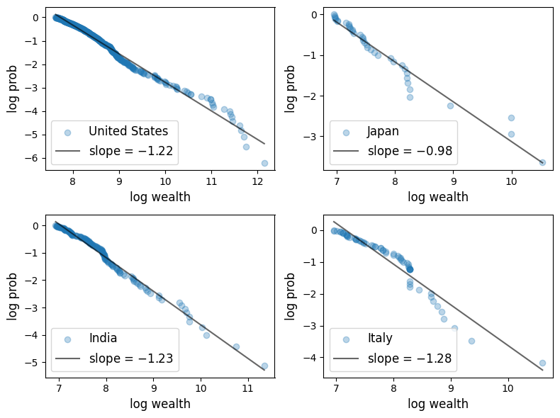
Figure 14:Wealth distribution (Forbes billionaires in 2020)
21.3.4GDP
Of course, not all cross-sectional distributions are heavy-tailed.
Here we show cross-country per capita GDP.
Source
# get gdp and gdp per capita for all regions and countries in 2021

variable_code = ['NY.GDP.MKTP.CD', 'NY.GDP.PCAP.CD']
variable_names = ['GDP', 'GDP per capita']

df_gdp1 = extract_wb(varlist=variable_code,
                     c="all_countries",
                     s="2021",
                     e="2021",
                     varnames=variable_names)
df_gdp1.dropna(inplace=True)
Source
fig, axes = plt.subplots(1, 2, figsize=(8.8, 3.6))

for name, ax in zip(variable_names, axes):
    empirical_ccdf(np.asarray(df_gdp1[name]).astype("float64"), ax, add_reg_line=False, label=name)

plt.show()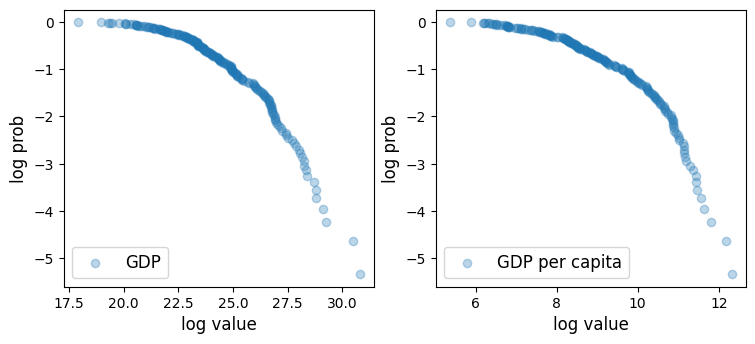
Figure 15:GDP per capita distribution
The plot is concave rather than linear, so the distribution has light tails.
One reason is that this is data on an aggregate variable, which involves some averaging in its definition.
Averaging tends to eliminate extreme outcomes.
21.4Failure of the LLN
One impact of heavy tails is that sample averages can be poor estimators of the underlying mean of the distribution.
To understand this point better, recall our earlier discussion of the law of large numbers, which considered IID with common distribution
If is finite, then the sample mean satisfies
where is the common mean of the sample.
The condition holds in most cases but can fail if the distribution is very heavy-tailed.
For example, it fails for the Cauchy distribution.
Let’s have a look at the behavior of the sample mean in this case, and see whether or not the LLN is still valid.
from scipy.stats import cauchy

np.random.seed(1234)
N = 1_000

distribution = cauchy()

fig, ax = plt.subplots()
data = distribution.rvs(N)

# Compute sample mean at each n
sample_mean = np.empty(N)
for n in range(1, N):
    sample_mean[n] = np.mean(data[:n])

# Plot
ax.plot(range(N), sample_mean, alpha=0.6, label='$\\bar{X}_n$')
ax.plot(range(N), np.zeros(N), 'k--', lw=0.5)
ax.set_xlabel(r"$n$")
ax.legend()

plt.show()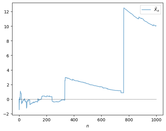
Figure 16:LLN failure
The sequence shows no sign of converging.
We return to this point in the exercises.
21.5Why do heavy tails matter?
We have now seen that
- heavy tails are frequent in economics and
- the law of large numbers fails when tails are very heavy.
But what about in the real world? Do heavy tails matter?
Let’s briefly discuss why they do.
21.5.1Diversification
One of the most important ideas in investing is using diversification to reduce risk.
This is a very old idea --- consider, for example, the expression “don’t put all your eggs in one basket”.
To illustrate, consider an investor with one dollar of wealth and a choice over assets with payoffs .
Suppose that returns on distinct assets are independent and each return has mean μ and variance .
If the investor puts all wealth in one asset, say, then the expected payoff of the portfolio is μ and the variance is .
If instead the investor puts share of her wealth in each asset, then the portfolio payoff is
Try computing the mean and variance.
You will find that
- The mean is unchanged at μ, while
- the variance of the portfolio has fallen to .
Diversification reduces risk, as expected.
But there is a hidden assumption here: the variance of returns is finite.
If the distribution is heavy-tailed and the variance is infinite, then this logic is incorrect.
For example, we saw above that if every is Cauchy, then so is .
This means that diversification doesn’t help at all!
21.5.2Fiscal policy
The heaviness of the tail in the wealth distribution matters for taxation and redistribution policies.
The same is true for the income distribution.
For example, the heaviness of the tail of the income distribution helps determine how much revenue a given tax policy will raise.
21.6Classifying tail properties
Up until now we have discussed light and heavy tails without any mathematical definitions.
Let’s now rectify this.
We will focus our attention on the right hand tails of nonnegative random variables and their distributions.
The definitions for left hand tails are very similar and we omit them to simplify the exposition.
21.6.1Light and heavy tails
A distribution with density on is called heavy-tailed if
We say that a nonnegative random variable is heavy-tailed if its density is heavy-tailed.
This is equivalent to stating that its moment generating function is infinite for all .
For example, the log-normal distribution is heavy-tailed because its moment generating function is infinite everywhere on .
The Pareto distribution is also heavy-tailed.
Less formally, a heavy-tailed distribution is one that is not exponentially bounded (i.e. the tails are heavier than the exponential distribution).
A distribution on is called light-tailed if it is not heavy-tailed.
A nonnegative random variable is light-tailed if its distribution is light-tailed.
For example, every random variable with bounded support is light-tailed. (Why?)
As another example, if has the exponential distribution, with cdf for some , then its moment generating function is
In particular, is finite whenever , so is light-tailed.
One can show that if is light-tailed, then all of its moments are finite.
Conversely, if some moment is infinite, then is heavy-tailed.
The latter condition is not necessary, however.
For example, the lognormal distribution is heavy-tailed but every moment is finite.
21.7Further reading
For more on heavy tails in the wealth distribution, see e.g., Vilfredo (1896) and Benhabib & Bisin (2018).
For more on heavy tails in the firm size distribution, see e.g., Axtell (2001), Gabaix (2016).
For more on heavy tails in the city size distribution, see e.g., Rozenfeld et al. (2011), Gabaix (2016).
There are other important implications of heavy tails, aside from those discussed above.
For example, heavy tails in income and wealth affect productivity growth, business cycles, and political economy.
For further reading, see, for example, Acemoglu & Robinson (2002), Glaeser et al. (2003), Bhandari et al. (2018) or Ahn et al. (2018).
21.8Exercises
Solution to Exercise 2
Solution to Exercise 3
from scipy.stats import pareto

np.random.seed(11)

n = 120
alphas = [1.15, 1.50, 1.75]

fig, axes = plt.subplots(3, 1, figsize=(6, 8))

for (a, ax) in zip(alphas, axes):
    ax.set_ylim((-5, 50))
    data = pareto.rvs(size=n, scale=1, b=a)
    ax.plot(list(range(n)), data, linestyle='', marker='o', alpha=0.5, ms=4)
    ax.vlines(list(range(n)), 0, data, lw=0.2)
    ax.set_title(f"Pareto draws with $\\alpha = {a}$", fontsize=11)

plt.subplots_adjust(hspace=0.4)

plt.show()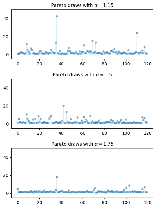
Solution to Exercise 4
To do the exercise, we need to choose the parameters μ and σ of the lognormal distribution to match the mean and median of the Pareto distribution.
Here we understand the lognormal distribution as that of the random variable when is standard normal.
The mean and median of the Pareto distribution (2) with are
Using the corresponding expressions for the lognormal distribution leads us to the equations
which we solve for μ and σ given .
Here is the code that generates the two samples, produces the violin plot and prints the mean and standard deviation of the two samples.
num_firms = 100_000
num_years = 10
tax_rate = 0.15
r = 0.05

β = 1 / (1 + r)    # discount factor

x_bar = 1.0
α = 1.05

def pareto_rvs(n):
    "Uses a standard method to generate Pareto draws."
    u = np.random.uniform(size=n)
    y = x_bar / (u**(1/α))
    return y
Let’s compute the lognormal parameters:
μ = np.log(2) / α
σ_sq = 2 * (np.log(α/(α - 1)) - np.log(2)/α)
σ = np.sqrt(σ_sq)
Here’s a function to compute a single estimate of tax revenue for a particular
choice of distribution dist.
def tax_rev(dist):
    tax_raised = 0
    for t in range(num_years):
        if dist == 'pareto':
            π = pareto_rvs(num_firms)
        else:
            π = np.exp(μ + σ * np.random.randn(num_firms))
        tax_raised += β**t * np.sum(π * tax_rate)
    return tax_raised
Now let’s generate the violin plot.
num_reps = 100
np.random.seed(1234)

tax_rev_lognorm = np.empty(num_reps)
tax_rev_pareto = np.empty(num_reps)

for i in range(num_reps):
    tax_rev_pareto[i] = tax_rev('pareto')
    tax_rev_lognorm[i] = tax_rev('lognorm')

fig, ax = plt.subplots()

data = tax_rev_pareto, tax_rev_lognorm

ax.violinplot(data)

plt.show()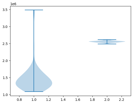
Finally, let’s print the means and standard deviations.
tax_rev_pareto.mean(), tax_rev_pareto.std()(np.float64(1458729.0546623734), np.float64(406089.3613661567))tax_rev_lognorm.mean(), tax_rev_lognorm.std()(np.float64(2556174.8615230713), np.float64(25586.44456513965))Looking at the output of the code, our main conclusion is that the Pareto assumption leads to a lower mean and greater dispersion.
Solution to Exercise 5
- Mandelbrot, B. (1963). The variation of certain speculative prices. The Journal of Business, 36(4), 394–419.
- Rachev, S. T. (2003). Handbook of heavy tailed distributions in finance: Handbooks in finance (Vol. 1). Elsevier.
- Vilfredo, P. (1896). Cours d’économie politique. Rouge, Lausanne, 2.
- Benhabib, J., & Bisin, A. (2018). Skewed wealth distributions: Theory and empirics. Journal of Economic Literature, 56(4), 1261–1291.
- Axtell, R. L. (2001). Zipf distribution of US firm sizes. Science, 293(5536), 1818–1820.
- Gabaix, X. (2016). Power laws in economics: An introduction. Journal of Economic Perspectives, 30(1), 185–206.
- Rozenfeld, H. D., Rybski, D., Gabaix, X., & Makse, H. A. (2011). The area and population of cities: New insights from a different perspective on cities. American Economic Review, 101(5), 2205–2225.
- Acemoglu, D., & Robinson, J. A. (2002). The Political Economy of the Kuznets curve. Review of Development Economics, 6(2), 183–203.
- Glaeser, E., Scheinkman, J., & Shleifer, A. (2003). The Injustice of Inequality. Journal of Monetary Economics, 50(1), 199–222.
- Bhandari, A., Evans, D., Golosov, M., & Sargent, T. J. (2018). Inequality, Business Cycles, and Monetary-Fiscal Policy [Techreport]. National Bureau of Economic Research.
- Ahn, S., Kaplan, G., Moll, B., Winberry, T., & Wolf, C. (2018). When Inequality Matters for Macro and Macro Matters for Inequality. NBER Macroeconomics Annual, 32(1), 1–75.
- Fujiwara, Y., Di Guilmi, C., Aoyama, H., Gallegati, M., & Souma, W. (2004). Do Pareto–Zipf and Gibrat laws hold true? An analysis with European firms. Physica A: Statistical Mechanics and Its Applications, 335(1–2), 197–216.
- Kondo, I., Lewis, L. T., & Stella, A. (2018). On the US Firm and Establishment Size Distributions [Techreport]. SSRN.
- Schluter, C., & Trede, M. (2019). Size distributions reconsidered. Econometric Reviews, 38(6), 695–710.

Creative Commons License – This work is licensed under a Creative Commons Attribution-ShareAlike 4.0 International.